RD-E: 1200 Jumping Bicycle
After a quasi-static pre-loading using gravity, a dummy cyclist rides along a plane, then jumps down onto a lower plane. Sensors are used to simulate the scenario in terms of time.
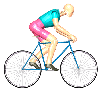
Figure 1.
Options and Keywords Used
- Shell, brick, beam, truss, general spring, and beam
- Sensors on rigid bodies (/SENSOR and /RBODY) and monitored volumes (perfect gas) (/MONVOL/GAS)
- Quasi-static load treatment (gravity) (/GRAV), kinetic relaxation (/KEREL), restart file
- Dummy and hierarchy organization
- TYPE7 interface auto-impacting (/INTER/TYPE7) and rigid wall (infinite plane and parallelogram) (/RWALL)
- Linear elastic law (/MAT/LAW1 (ELAST)) and Johnson-Cook law (/MAT/LAW2 (PLAS_JOHNS))
- Added mass (/ADMAS)
- Initial velocity (/INIVEL)
- A fixed infinite plane (floor)
- A fixed parallelogram (springboard)
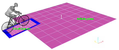
Figure 2. Position of the Rigid Walls
The characteristics of the parallelogram plane are: 2013 mm x 1200 mm. Both rigid walls are tied to allow the wheels to turn.
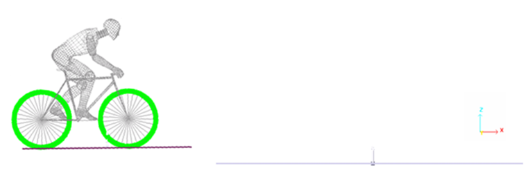
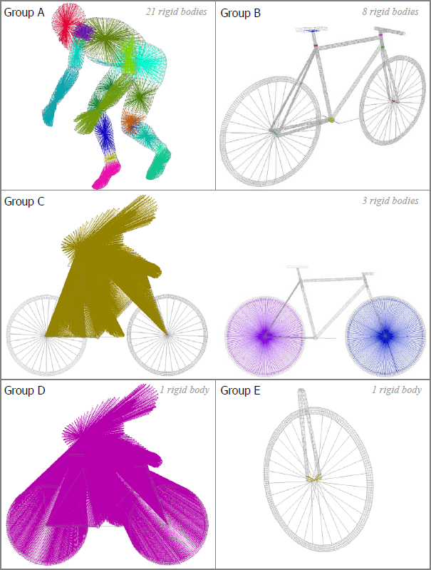
Figure 4. Classification of Rigid Bodies (group)
The inertias of rigid bodies are set in local skew frames for groups A, C and D.
- Rigid body activation/deactivation
- Groups A and B
- The rigid bodies are activated during pre-loading up to equilibrium then applied to the initial velocity start. They are activated again just before the impact of the bike on the inferior plane.
- Group C
- Three rigid bodies include the dummy, the frame and both wheels (not including the tires). This configuration allows just the wheels to turn, taking into account the active tires action on the plane. This rigid body is activated while the bike is running on the springboard.
- Group D
- This global rigid body, including all nodes of model is activated as long as the bike is in the free fly phase and is deactivated just before impact on the floor.
- Group E
- This rigid body is activated before impact ensures the stiffness level of the lower fork.
A 8333 mms-1(30 km/h) initial velocity (/INIVEL) is applied to all nodes of the model (bicycle and cyclist) in a parallel direction to the high plane at time t = 0.004 s. This initial condition is defined in the Engine file *_0002.rad (start time: 0.004 s) which is run after the quasi-static equilibrium with gravity loading.
- /INIV/TRA/X/1
- initial translational velocities in direction x
- 8333
- of 8333 mm/s
- 1 338000
- on node 1 to 338000
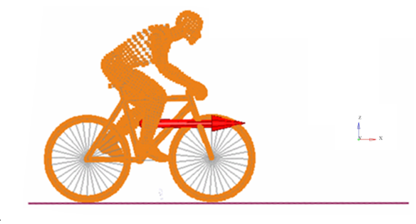
Figure 5. Initial Translational Velocities of the Model Bike/Man (30 km/h) at t = 0.004 s
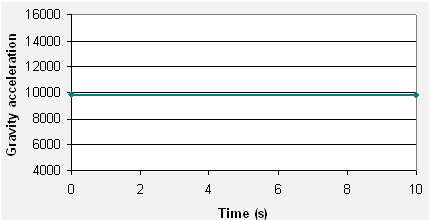
Figure 6. Gravity Function (-9810 mm/s-2)
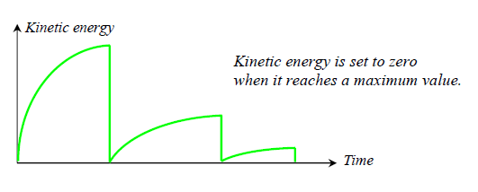
Figure 7. Kinetic Relaxation Method
- TIME
- Activated with time
- DIST
- Activated with nodal distance
- INTER
- Activated after impact on rigid wall
- SENSOR
- Activated with sensor IS1 and deactivated with sensor IS2
- NOT
- ON as long as sensor IS1 is OFF
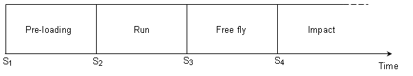
Figure 8. Events Definition for the Activations and Deactivations of Sensors
At the beginning of the simulation (time=0), the rigid bodies are automatically set to ON, as long as the sensors are not active. Thus, in order to deactivate the rigid bodies at the first cycle, active sensors at time t=0 should be used. Consequently, the rigid bodies are active when the sensors are not active.
| Name | Type | Definition | Rigid Body's Group using Sensor |
|---|---|---|---|
| S1 | TIME | Time 0s. | - |
| S2 | DIST | Distance between rear hubs and extremity of springboard equal to 1810 mm. | - |
| S3 | DIST | Distance between rear hubs and extremity of springboard equal to 345 mm. | - |
| S4 | RWALL | When the infinite rigid wall is impacted. | - |
| SEN(S2,S3) | SEN | Activated with S2 and deactivated with S3 | - |
| SEN(S3,S4) | SEN | Activated with S3 and deactivated with S4 | - |
| SEN(S2,S4) | SEN | Activated with S2 and deactivated with S4 | Group A/B |
| NOT(SEN(S2,S3)) | NOT | Deactivated with S2 and activated with S3 | Group C |
| NOT(SEN(S3,S4)) | NOT | Deactivated with S3 and activated with S4 | Group D |
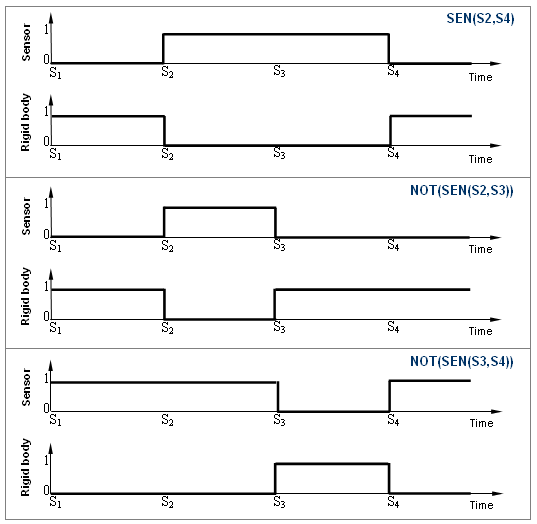
Figure 9. Activation and Deactivation Zones of Sensors and Rigid Bodies
Input Files
- Jumping_bicycle
- <install_directory>/hwsolvers/demos/radioss/example/12_Bicycle/Bike/BIKERC*
Model Description
The purpose of this example is to set up a demonstration in which sensors and restart files are used to allow the change of a problem over time.
- positioning the cyclist under the gravity effect
- running the bicycle on the high plane
- free fly
- the impact on the ground
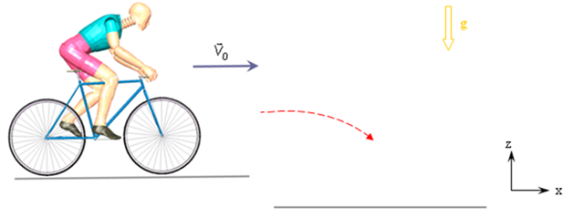
Figure 10.
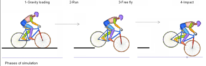
Figure 11.
Model Method
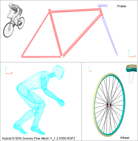
Figure 12. Meshes of the Models Main Parts
- Steel Spokes Material Properties
- Young's modulus
- 210000
- Poisson's ratio
- 0.3
- Density
- 7.9x10⁻⁹
- Yield stress
- 185.4
- Hardening parameter
- 540
- Hardening exponent
- 0.32
- Aluminum Frame Material Properties
- Young's modulus
- 60400
- Poisson's ratio
- 0.33
- Density
- 2.7x10⁻⁹
- Yield stress
- 90.27
- Hardening parameter
- 223.14
- Hardening exponent
- 0.375
| Parts | Properties | Materials | |
|---|---|---|---|
| Bike | Frame | Shell Q4 - 3 mm | Aluminum - Law 2 |
| Spokes | Truss - 2 mm2 | Steel - Law 2 | |
| Rim | Shell Q4 - 3 mm | Aluminum - Law 2 | |
| Tires | Shell QEPH - 3 mm | Rubber - Law 1 | |
| Hubs | Beam - 900 mm2 | Steel - Law 2 | |
| Saddle | Brick | Foam - Law 1 | |
| Pedals | Beam - 900 mm2 | Steel - Law 2 | |
| Tube of saddle | Shell Q4 - 3 mm | Aluminum - Law 2 | |
| Dummy | Body (limbs) | Shell Q4 - 3 mm | Law 1 |
| Joints | Spring (8) | - |
- Bike model
- 6 subsets comprising 23 parts
- Dummy model
- 11 subsets comprising 38 parts
Monitored Volumes / Perfect Gas
A perfect gas monitored volume with /MONVOL/GAS is defined to model the pressure in the tires. For further details about monitored volumes, refer to GAS Type in the Radioss Theory Manual.
- External pressure Pext
- 0.1
- Initial internal pressure Pini
- Front tire: 0.75
- Gas constant
- 1.4
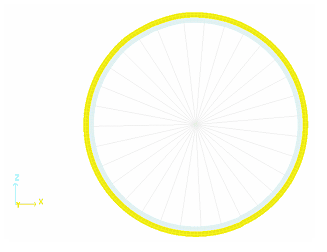
Figure 13. Visualization of a Monitored Volume (yellow part)
- Quasi-static loading: gravity effect on initial static equilibrium
The quasi-static solution of gravity loading on structure deformation corresponds to the steady state part of the transient response. It describes the pre-loading case before the dynamic analysis. Therefore, the simulation is divided into two phases: quasi-static response (structure subjected to the gravity) and dynamic behavior (run, jump and landing). The solution is obtained from kinetic relaxation (/KEREL). Gravity is defined by /GRAV.
- Contacts modelingThe TYPE7 interface using the penalty method serves to model contacts between the dummy cyclist and the bike. With contact in /RWALL to treat the landing of the bike. Figure 14 illustrates the description of the interface.
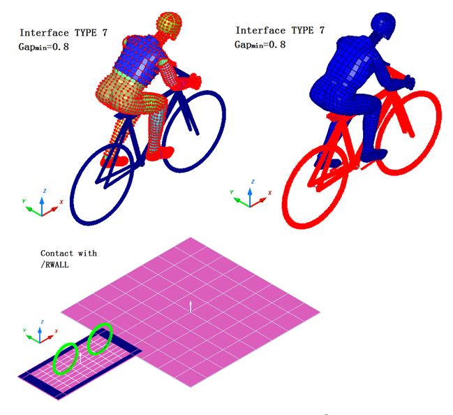
Figure 14. Contacts Modeling with TYPE7 Interface (Penalty Method) and /RWALL
- Links between man and bicycle
- Stiffness (TX, TY and TZ)
- 50
- Mass
- 1e-10
- Inertia
- 1e-5
- Left hand: Z = 20 mm
- Right hand: Z = 20 mm
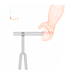
Figure 15. Link Right Hand/Handlebar (TYPE8 Springs) - Dummy joints
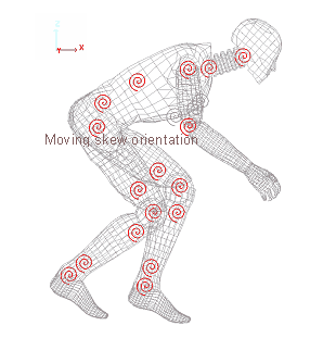
Figure 16. TYPE8 Springs
The general TYPE8 springs, characterize a spherical hinge with a stiffness given for each DOF. Directions are local and attached to a moving skew frame. Two coinciding nodes define a spring.
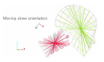
Figure 17. Connection Rigid Body - Spring TYPE8 - Rigid Body
- Wheel rotation
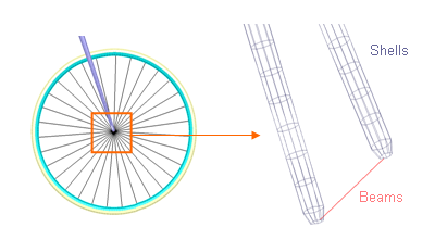
Figure 18. Wheel/Forks Junction
Results
The elements included in a rigid body are deactivated. Therefore, the element flags saved in /TH/RBODY provide information on the activation and deactivation of rigid bodies during simulation.
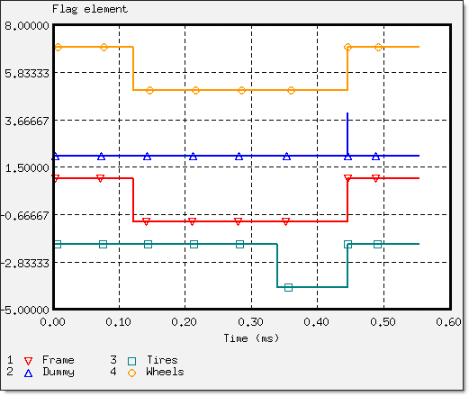
Figure 19. Activation and Deactivation of Main Model Parts (elements flag ON/OFF)
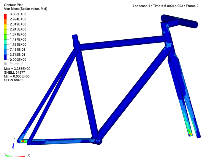
Figure 20. Distribution of the von Mises Stress on the Frame after Quasi-static Loading
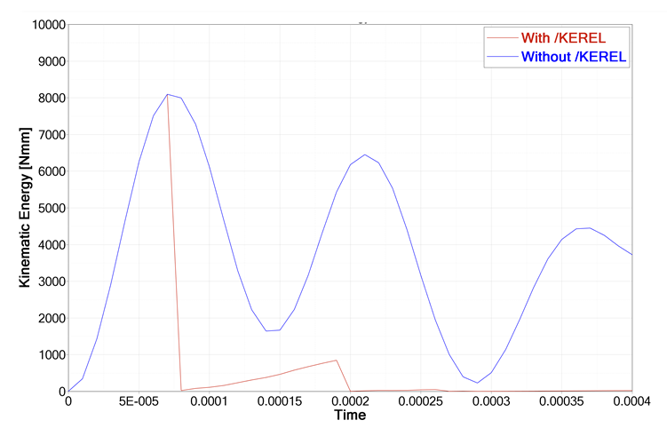
Figure 21. Kinetic Relaxation Effect on Kinetic Energy with /KEREL
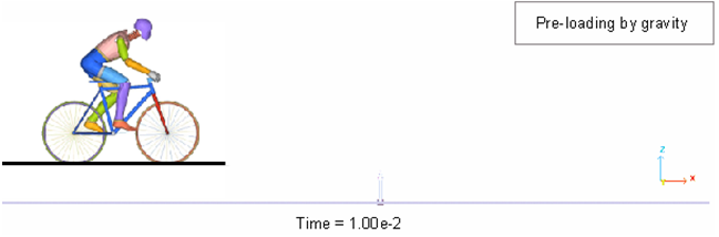
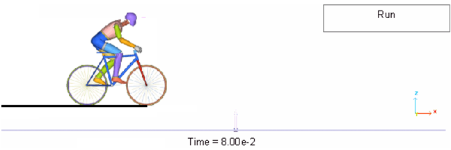
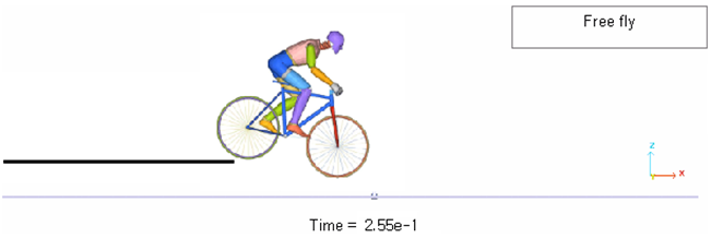
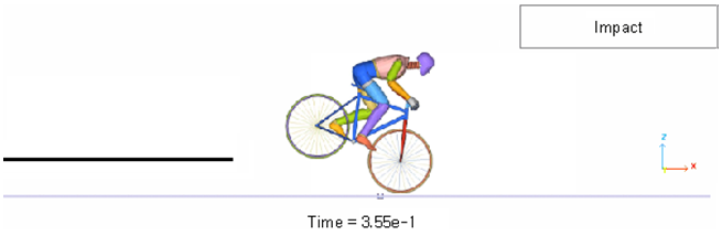
Figure 23. Dummy Cyclist during Impact on the Ground (shoes not attached)
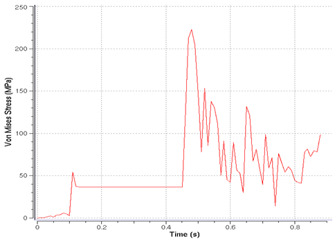
Figure 24. Variation of von Mises Stress for a Shell Element of the Frame