RD-E: 2000 Ice Cube

Ice cube dropping on two sliding channels.
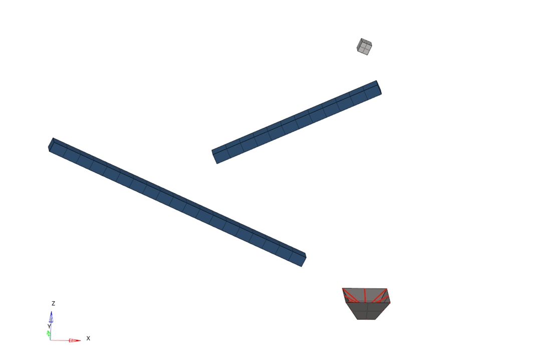

rad_ex_20_cube
Figure 1.

The subject in this example demonstrates the falling and sliding of an ice cube on to sloped beams using an explicit transient dynamic analysis for deformable, free-flying objects. The impact and rebound are modeled using penalty contact algorithms.

The Contact between the ice cube, the beams, and the cup are modeled using different penalty contact interfaces (/INTER/TYPE7, /INTER/TYPE24 and /INTER/TYPE25). The ice cube and the beams are modeled using hexahedron elements. The cup is modeled with standard shell elements.

Options and Keywords Used

  • Boundary conditions on node groups for translational and rotational motion (/BCS):
    • The ice cube nodes are constrained in the Y translation.
    • The bottom nodes of the beams are constrained in all directions.
    • The cup is constrained in all directions
  • Gravity (/GRAV):
    • A gravity load (g = 9.81 m/s2) in the Z-direction is applied on the ice cube’s nodes
  • Interfaces: Three different node to surface penalty contact interfaces are compared with each other. For each model, the ice cube is the secondary and the main is the beams and cup.
    • /INTER/TYPE7 interface uses the penalty method with an initial gap of 0.1. Ice cube nodes are the secondary and the main surface is defined using the upper surface of the beams and the cup. To replicate surface to surface contact, a second TYPE7 contact is created with the ice cube as main surface and the beams and cup as secondary nodes. The interface stiffness is the minimum value of the main and secondary stiffness (Istf = 4). The TYPE7 interface is a general impact interface with a nonlinear stiffness. In case of high impact speed or contacts with a small gap, the time step can be reduced because the contact stiffness will increase if the secondary node penetrates closer to the main surface.
    • /INTER/TYPE24 interface uses the penalty method without any contact gap between the solid elements. A surface to surface contact is defined where the ice cube is defined as a secondary surface and the main surface is defined using the upper surface of the beams and the cup. The interface stiffness is the minimum value of the main and secondary stiffness (Istf = 4). The TYPE24 interface is a general nodes-to-surface contact interface using the penalty method with a constant interface stiffness which means there is no reduction in time step due to secondary node penetration. Three different input types can be used: single surface, surface to surface, or nodes to surface. This contact is typically used for drop test simulations.
    • /INTER/TYPE25 is very similar to TYPE24 in its definition and algorithm. However, it is being developed for crash impact simulations and; therefore, has a few different options and algorithms.
  • /PROP/TYPE1 (SHELL)
  • /PROP/TYPE14 (SOLID)

Input Files

The input file used in this example includes:
  • <install_directory>/hwsolvers/demos/radioss/example/20_Cube/

Model Description

This problem provides a comparison of different contact interfaces that allow sliding contact between an ice cube and steel beams.

The cube is submitted to gravity and slides on declined fixed beams. Finally, it is collected in a cup. The width of the cube is 30 mm and the dimensions of the beams are 40 x 30 x 500 mm.

The ice cube is modeled as a simple elasto-plastic material using /MAT/LAW2, with the following characteristics:
Initial density
9.16e-10 M g m m 3 MathType@MTEF@5@5@+= feaagKart1ev2aqatCvAUfeBSjuyZL2yd9gzLbvyNv2CaerbuLwBLn hiov2DGi1BTfMBaeXatLxBI9gBaerbd9wDYLwzYbItLDharqqtubsr 4rNCHbGeaGqiVu0Je9sqqrpepC0xbbL8F4rqqrFfpeea0xe9Lq=Jc9 vqaqpepm0xbba9pwe9Q8fs0=yqaqpepae9pg0FirpepeKkFr0xfr=x fr=xb9adbaqaaeGaciGaaiaabeqaamaabaabaaGcbaWaaSaaaeaaca WGnbGaam4zaaqaaiaad2gacaWGTbWaaWbaaSqabeaacaaIZaaaaaaa aaa@3A93@
Young's modulus
8996 [ MPa ] MathType@MTEF@5@5@+= feaagKart1ev2aqatCvAUfeBSjuyZL2yd9gzLbvyNv2CaerbuLwBLn hiov2DGi1BTfMBaeXatLxBI9gBaerbd9wDYLwzYbItLDharqqtubsr 4rNCHbGeaGqiVu0Je9sqqrpepC0xbbL8F4rqGqFfpeea0xe9vq=Jb9 vqpeea0xd9q8qiYRWxGi6xij=hbba9q8aq0=yq=He9q8qiLsFr0=vr 0=vr0db8meaabaqaciGacaGaaeqabaWaaeaaeaaakeaadaWadaqaai Gac2eacaGGqbGaaiyyaaGaay5waiaaw2faaaaa@3BE6@
Poisson's ratio
0.3
Yield Stress, SIGY
1.0 [ MPa ] MathType@MTEF@5@5@+= feaagKart1ev2aqatCvAUfeBSjuyZL2yd9gzLbvyNv2CaerbuLwBLn hiov2DGi1BTfMBaeXatLxBI9gBaerbd9wDYLwzYbItLDharqqtubsr 4rNCHbGeaGqiVu0Je9sqqrpepC0xbbL8F4rqGqFfpeea0xe9vq=Jb9 vqpeea0xd9q8qiYRWxGi6xij=hbba9q8aq0=yq=He9q8qiLsFr0=vr 0=vr0db8meaabaqaciGacaGaaeqabaWaaeaaeaaakeaadaWadaqaai Gac2eacaGGqbGaaiyyaaGaay5waiaaw2faaaaa@3BE6@
Hardening parameter, b
4.0 [ MPa ] MathType@MTEF@5@5@+= feaagKart1ev2aqatCvAUfeBSjuyZL2yd9gzLbvyNv2CaerbuLwBLn hiov2DGi1BTfMBaeXatLxBI9gBaerbd9wDYLwzYbItLDharqqtubsr 4rNCHbGeaGqiVu0Je9sqqrpepC0xbbL8F4rqGqFfpeea0xe9vq=Jb9 vqpeea0xd9q8qiYRWxGi6xij=hbba9q8aq0=yq=He9q8qiLsFr0=vr 0=vr0db8meaabaqaciGacaGaaeqabaWaaeaaeaaakeaadaWadaqaai Gac2eacaGGqbGaaiyyaaGaay5waiaaw2faaaaa@3BE6@
Hardening exponent, n
0.5
The material used for the beams and the cup is steel and follows an isotropic elasto-plastic material (/MAT/LAW2) with the Johnson-Cook plasticity model, having the following characteristics:
Initial density
7.8e-09 M g m m 3 MathType@MTEF@5@5@+= feaagKart1ev2aqatCvAUfeBSjuyZL2yd9gzLbvyNv2CaerbuLwBLn hiov2DGi1BTfMBaeXatLxBI9gBaerbd9wDYLwzYbItLDharqqtubsr 4rNCHbGeaGqiVu0Je9sqqrpepC0xbbL8F4rqqrFfpeea0xe9Lq=Jc9 vqaqpepm0xbba9pwe9Q8fs0=yqaqpepae9pg0FirpepeKkFr0xfr=x fr=xb9adbaqaaeGaciGaaiaabeqaamaabaabaaGcbaWaaSaaaeaaca WGnbGaam4zaaqaaiaad2gacaWGTbWaaWbaaSqabeaacaaIZaaaaaaa aaa@3A93@
Young's modulus
210000 [ MPa ] MathType@MTEF@5@5@+= feaagKart1ev2aqatCvAUfeBSjuyZL2yd9gzLbvyNv2CaerbuLwBLn hiov2DGi1BTfMBaeXatLxBI9gBaerbd9wDYLwzYbItLDharqqtubsr 4rNCHbGeaGqiVu0Je9sqqrpepC0xbbL8F4rqGqFfpeea0xe9vq=Jb9 vqpeea0xd9q8qiYRWxGi6xij=hbba9q8aq0=yq=He9q8qiLsFr0=vr 0=vr0db8meaabaqaciGacaGaaeqabaWaaeaaeaaakeaadaWadaqaai Gac2eacaGGqbGaaiyyaaGaay5waiaaw2faaaaa@3BE6@
Poisson's ratio
0.3
Yield stress, SIGY
200 [ MPa ] MathType@MTEF@5@5@+= feaagKart1ev2aqatCvAUfeBSjuyZL2yd9gzLbvyNv2CaerbuLwBLn hiov2DGi1BTfMBaeXatLxBI9gBaerbd9wDYLwzYbItLDharqqtubsr 4rNCHbGeaGqiVu0Je9sqqrpepC0xbbL8F4rqGqFfpeea0xe9vq=Jb9 vqpeea0xd9q8qiYRWxGi6xij=hbba9q8aq0=yq=He9q8qiLsFr0=vr 0=vr0db8meaabaqaciGacaGaaeqabaWaaeaaeaaakeaadaWadaqaai Gac2eacaGGqbGaaiyyaaGaay5waiaaw2faaaaa@3BE6@
Hardening parameter, b
400 [ MPa ] MathType@MTEF@5@5@+= feaagKart1ev2aqatCvAUfeBSjuyZL2yd9gzLbvyNv2CaerbuLwBLn hiov2DGi1BTfMBaeXatLxBI9gBaerbd9wDYLwzYbItLDharqqtubsr 4rNCHbGeaGqiVu0Je9sqqrpepC0xbbL8F4rqGqFfpeea0xe9vq=Jb9 vqpeea0xd9q8qiYRWxGi6xij=hbba9q8aq0=yq=He9q8qiLsFr0=vr 0=vr0db8meaabaqaciGacaGaaeqabaWaaeaaeaaakeaadaWadaqaai Gac2eacaGGqbGaaiyyaaGaay5waiaaw2faaaaa@3BE6@
Hardening exponent, n
0.5

Units: mm, s, Mg, N, MPa

Results

Figure 2 shows the trajectory of the ice cube for the three different contact interfaces, which was created using the Trace component option in HyperView. The impact of the cube on the first beam is very similar for all three contact interfaces. As the minor differences accumulate, the motion becomes different after the impact with the second beam.

rad_ex_fig_20-3
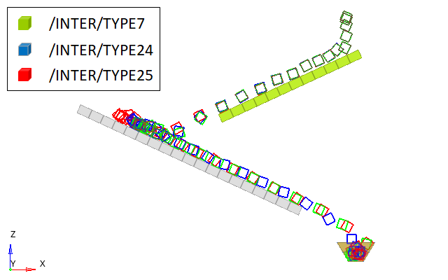
Figure 2. Trajectory of the Ice Cube using Interface TYPE7, TYPE24 and TYPE25
Figure 3 shows a comparison of the total reaction forces for the three interfaces. The differences in the results are to be expected since all interfaces have different formulations. Those differences accumulate resulting in different motion toward the end of the simulation.

rad_ex_fig_20-4
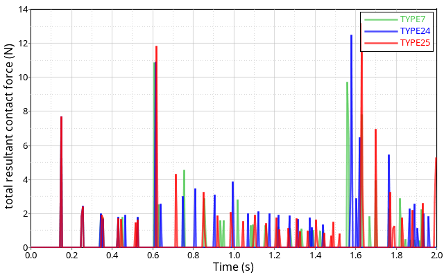
Figure 3. Comparison of the Reaction Forces of the Ice Cube on the Beams