RD-E: 2100 Cam
The modeling of a camshaft, which takes the engine's rotary motion and translates it into linear motion for operating the intake and exhaust valves, is studied.
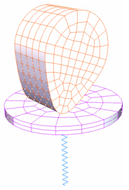
Figure 1.
Options and Keywords Used
- Linear/quadratic elements and quadratic surface contact
- BRIC20 elements (/BRIC20)
- SHEL16 elements (/SHEL16)
- Initial velocities around axis (/INIVEL/AXIS)
- Spring element (/PROP/TYPE4 (SPRING))
- Penalty/Lagrangian contact Interfaces (/INTER/LAGMUL/TYPE16 and /INTER/LAGMUL/TYPE7)
- Rigid bodies: In order to apply a constant angular velocity to the cam, a
rigid body is created over the internal nodes, as shown in Figure 2. The
main node is moved to the camshaft axis. To attach the valve head to the spring, another rigid body is created to distribute the internal spring force over several nodes.
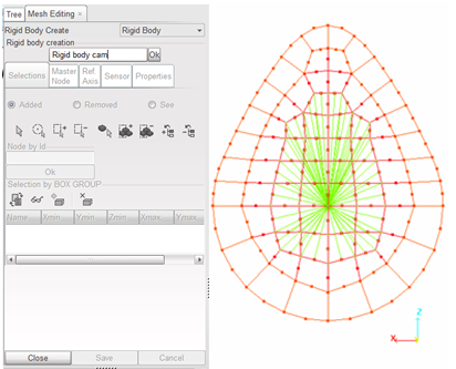
Figure 2. Rigid Body Cam - Boundary conditions:
- Main node of the cam is blocked, except when rotating around Y.
- Main node of the valve is blocked, except when translating around Z.
- One extremity of the spring is fixed to the valve, while the other
is blocked.
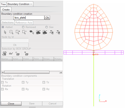
Figure 3. Boundary Condition on Valve
- Imposed velocity: A rotational velocity of 314 rad/s is imposed on the main
node of the rigid body. This velocity is activated by a temporal sensor,
with a short activation delay (Tdelay =0.0002s). This
sensor is necessary to avoid applying the initial and imposed velocities at
the same time.
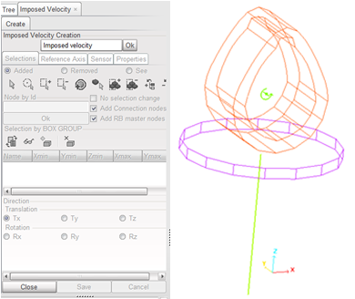
Figure 4. Imposed Velocity - Initial velocity: An initial rotational velocity is applied to all the cam's nodes, including the main node of the rigid body. You must define the origin (center of rotation) and the orientation vector.
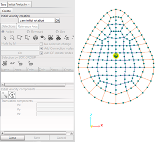
Figure 5. Initial Velocity - Interfaces: The TYPE16 interface simulates a contact between a quadratic
main surface and a group of nodes. In the case of contact between a curved
and a plane surface, the curved surface is defined as the main surface and
the nodes of the plane part are secondary.
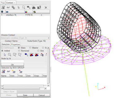
Figure 6. Interface TYPE6The TYPE7 interface works either with Penalty or with Lagrange multipliers. In its basic formulation, the interface simulates contact between two facetisated surfaces. The use of the Lagrange Multipliers method enables to precisely satisfy the kinematic contact without introducing a gap.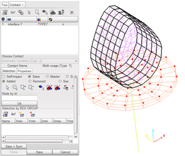
Figure 7. Interface TYPE7
Input Files
- Interface 16:
- Fine mesh
- <install_directory>/hwsolvers/demos/radioss/example/21_Cam/interface16/fine_mesh/I16S16FM*
- Coarse mesh
- <install_directory>/hwsolvers/demos/radioss/example/21_Cam/interface16/coarse_mesh/I16S16CM*
- Interface 7:
- Penalty method
- <install_directory>/hwsolvers/demos/radioss/example/21_Cam/interface7/penalty/second_cam/I7PMCAM*
- Lagrange multipliers
- <install_directory>/hwsolvers/demos/radioss/example/21_Cam/interface7/lagrange/second_cam/I7LMCAM*
- Friction
- <install_directory>/hwsolvers/demos/radioss/example/21_Cam/interface7/friction/I7PFMCAM*
Model Description
Modeling a contact between a plane and a curved surface uses a faceted curved surface. Interfaces 7 and 16 are compatible with the geometry of the problem and the faceting, are described and compared.
- The cam is 36 mm in length, with a maximum width of 14 mm and a thickness of 18 mm.
- The valve is 44 mm in diameter, with a thickness of 3 mm (Figure 8).
- The spring is 40 mm in length.
The following system is used: mm, s, kg, mN , KPa.
- Material Properties
- Initial density
- 7.8 x 10-06 Mkg/l
- Young's modulus
- 2.1 x 10+08 KPa
- Poisson ratio
- 0.3
- Yield stress
- 20000 KPa
- Hardening parameter
- 40000 KPa
- Hardening exponent
- 0.5
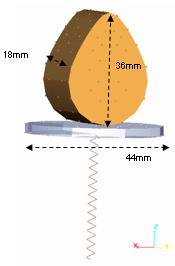
Figure 8. Geometry of the Problem
Model Method
The problem raised in this example is the modeling of an interface between a plane and a curved surface. In this case, using quadratic elements is the most appropriate.
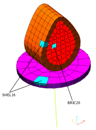
Figure 9. BRIC20 and SHEL16 Mesh
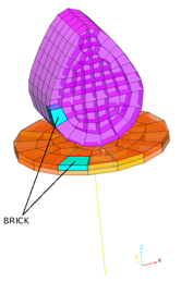
Figure 10. BRICK Elements Mesh
| l-l0 (mm) | -40 | 0 | 50 |
| Fspring 1 (mN) | -1.5 e+06 | -0.3 e+06 | 1.2 e+06 |
| Fspring 2 (mN) | -0.75 e+06 | -0.15 e+06 | 0.6 e+06 |
Results
At first, you are interested by the kinematics of the problem. The results obtained for velocity and acceleration at the main node of the rigid body's valve are thus compared.
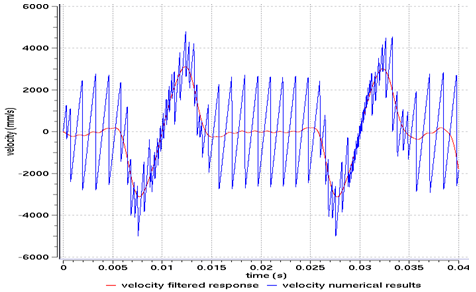
Figure 11. Vertical Velocity of the Main Node Valve for a TYPE7 Interface, using the Penalty Method
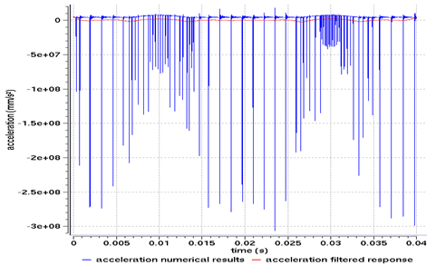
Figure 12. Vertical Acceleration of the Main Node Valve for a TYPE7 Interface, using the Penalty Method
The filtering quality depends on the number of samples which, in this case is the number of points computed by Radioss for each curve. Therefore, a low value for the /TFILE parameter in the Engine file (*_0001.rad) is used to obtain good results, especially for the acceleration curve.
In the following sections, only the filtered curves are represented in order to the compare different models.
Comparison of Interfaces
Figure 13 and Figure 14 represent velocity and acceleration curves for a model using a TYPE7 interface with the Penalty method. As for the main and secondary part definition, the results are slightly different.
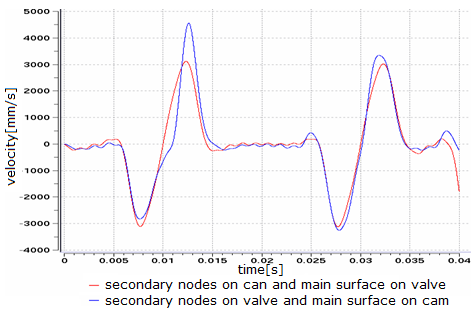
Figure 13. Vertical Velocity of the Valve's Main Node for a TYPE7 Interface, using the Penalty Method
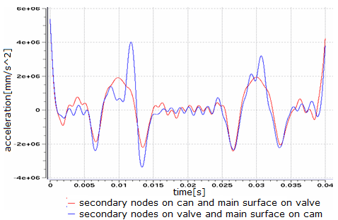
Figure 14. Vertical Acceleration of the Valve's Main Node for a TYPE7 Interface, using the Penalty Method
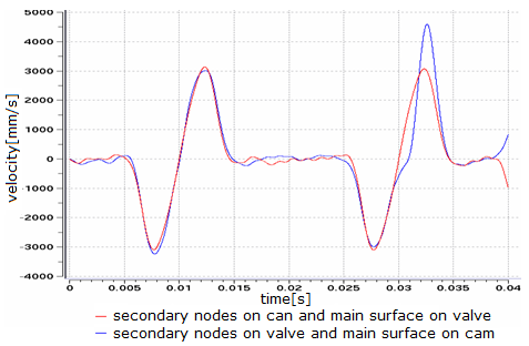
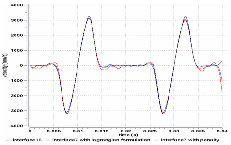
Figure 15. Vertical Velocity of the Valve's Main Node for a TYPE7 Interface, using the Lagrange Multipliers Method
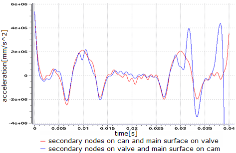
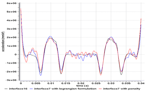
Figure 16. Vertical Acceleration of the Valve's Main Node for a TYPE7 Interface, using the Lagrange Multipliers Method
Even if using a TYPE7 interface with the Penalty or the Lagrange Multipliers method good results can be achieved, a quadratic mesh with the TYPE16 interface will enable the reduction of oscillations, due to facetisation.
Comparison of Meshes
- Fine Mesh:
- Cam
- 200 external SHEL16 elements, 250 internal BRIC20 elements
- Valve
- 88 SHEL16 elements
- Coarse Mesh:
- Cam
- 40 SHEL16 elements
- Valve
- 12 SHEL16 elements
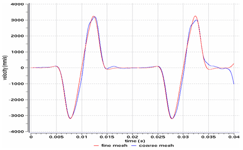
Figure 19. Vertical Velocity of the Valve's Main Node
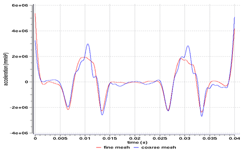
Figure 20. Vertical Acceleration of the Valve's Main Node
Although the coarser mesh amplifies the facetisation of the curved surfaced, the mesh density does not influence the results for velocity after filtering. However, the fine mesh provides better results for acceleration, having limited parasite oscillations for each node/surface contact.
Friction
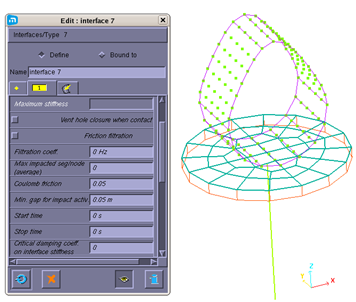
Figure 21. TYPE7 Interface using Penalty and Friction
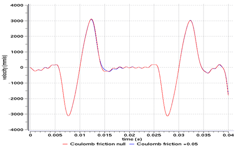
Figure 22. Vertical Velocity of the Valve's Main Node for a TYPE7 Interface, using the Penalty Method
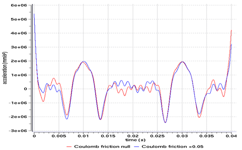
Figure 23. Vertical Acceleration of the Valve's Main Node for a TYPE7 Interface, using the Penalty Method
| Simulation | CPU (normalized) | Time Step |
|---|---|---|
| TYPE16 interface with fine mesh | 22,50 | 0.8365 x 10⁻⁷ |
| TYPE16 interface with coarse mesh | 1 | 0.207 x 10⁻⁶ |
| TYPE7 interface with
Penalty method (secondary nodes on cam and main surface on valve) |
1.65 | 0.2133 x 10⁻⁶ |
| TYPE7 interface with
penalty method (secondary nodes on valve and main surface on cam) |
1.75 | 0.2117 x 10⁻⁶ |
| TYPE7 interface with
Lagrange multipliers method (secondary nodes on cam and main surface on valve) |
1.68 | 0.2133 x 10⁻⁶ |
| TYPE7 interface with
Lagrange multipliers method (secondary nodes on valve and main surface on cam) |
1.69 | 0.2126 x 10⁻⁶ |
| TYPE7 interface with
Penalty method and friction (secondary nodes on cam and main surface on valve) |
1.66 | 0.2133 x 10⁻⁶ |
| TYPE7 interface with
Penalty method and friction (secondary nodes on valve and main surface on cam) |
1.65 | 0.2126 x 10⁻⁶ |
Conclusion
This example illustrated the ability of Radioss to model mechanisms, particularly in the case of this contact mechanism. Interface TYPE16 and TYPE7 can be used to model contact between plane and curved surfaces. The TYPE16 interface enables you to simulate contact between quadratic surfaces without using a gap and provides accurate results within a reasonable computation time. The TYPE7 interface allows a frictional modeling of the contact, needing little computation time and provides good simulation results.