RD-E: 0800 Hopkinson Bar
The high strain rate tensile behavior of the 7010 aluminum alloy is studied using the Hopkinson pressure bar technique (stress wave).
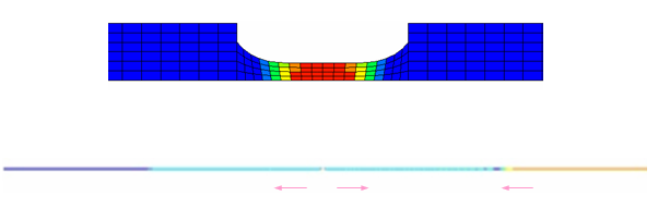
Figure 1.
Options and Keywords Used
- Axisymmetrical analysis (/ANALY) and quad elements
- High strain rate and Split Hopkinson Pressure Bar (SHPB)
- Wave propagation and stress pulse
- Elastic model (/MAT/LAW1 (ELAST)) and Johnson-Cook elasto-plastic model (/MAT/LAW2 (PLAS_JOHNS))
- Boundary conditions (/BCS)
- Imposed velocities (/IMPVEL)
Low extremity nodes of the output bar are fixed in the Z direction. The axisymmetrical condition on the revolutionary symmetry axis requires the blocking of the Y translation and X rotation.
The projectile is modeled using a steel cylinder with a fixed velocity in the direction Z. The required strain rate is taken into account by applying two imposed velocities, 1.7 ms-1 and 5.8 ms-1 in order to produce strain rate ranges in the of 80 s-1 and 900 s-1 (low and high rates) object.
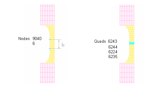
Figure 2. Nodes and Quads Saved for Time History
In the experiment, the strain gauge is attached to the object. In simulation, the true strain will be determined from 9040 and 6 nodes' relative Z displacements ( = 3.83638 mm).
The true stress can be given using two data sources. The first methodology consists of using the equation previously presented, based on the assumption of the one-dimensional propagation of bar-object forces. The engineering strain associated with the output stress wave is obtained from the Z displacement of nodes located on the output bar. The true plastic strain is extracted from the quads on the object, saved in the Time History file. True stress can also be measured directly from the Time History using the average of the Z stress quads 6243, 6244, 6224 and 6235. It should be noted that the section option is not an available option with the quad elements.
| High Rate Testing | ||
|---|---|---|
| True stress | Z stress average from quads saved in /TH | |
| True strain | ||
| True strain rate | ||
Input Files
- High_strain_rate
- <install_directory>/hwsolvers/demos/radioss/example/08_Hopkinson_Bar/High_strain_rate/SHPB_H*
- Low_strain_rate
- <install_directory>/hwsolvers/demos/radioss/example/08_Hopkinson_Bar/Low_strain_rate/SHPB_L*
Model Description
In order to model and predict the behavior of material during impact, the responses at very high strain rates should be studied.
The Split Hopkinson Bar is an inexpensive device for performing high strain-rate experiments. 1
- the striker bar
- the incident bar
- the transmission bar
- the drop bar
The object is sandwiched between the transmission and the incident bar. Assuming that the wave propagation in the bar is non-dispersive, the force and displacement upon contact between the bar and the object can be obtained from the strains measured through experience. In this example, the dynamic tensile behavior, achieved through experience of the 7010 aluminum alloy with a Split Hopkinson Pressure Bar (SHPB) is compared to numerical simulations. Two cases are studied at the strain rates of 80 s-1 (low rate) and 900 s-1 (high rate), respectively. At high strain rates, experience shows that the stress flow significantly increases by more than 30% with the strain rate increasing; thus demonstrating strain rate dependence in aluminum alloys in general. For the strain rates' range applied here, an existing Johnson-Cook model is used to describe the stress flow as a strain and strain rate function. Failure is not taken into account.
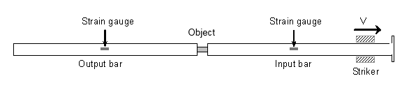
Figure 3. Hopkinson Bar Device
The objects material undergoes an isotropic elasto-plastic behavior which can be reproduced using a Johnson-Cook model (/MAT/LAW2). The steel bars and the striker follow a linear elastic law (/MAT/LAW1).
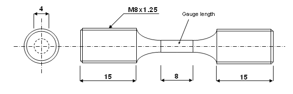
Figure 4. Object Geometry and Cross-section (dimensions in mm)
Taking into account the geometry's revolution symmetry, the material and the kinematic conditions, an axisymmetrical model is used (N2D3D = 1 in /ANALY set up in the Starter file). Y is the radial direction and Z is the axis of revolution.
Johnson-Cook Model
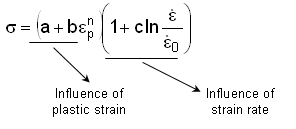
Figure 5.
- Strain rate
- Reference strain rate
- Plastic strain (true strain)
- a
- Yield stress
- b
- Hardening parameter
- n
- Hardening exponent
- c
- Strain rate coefficient
The two optional inputs, strain rate coefficient and reference strain rate, must be defined for each material in /MAT/LAW2 in order to take account of the strain rate effect on stress, that is the increase in stress when increasing the strain rate. The constants a, b and n define the shape of the strain-stress curve.
- Strain rates below 80 s-1
- Strain rates exceeding 80 s-1 up to 3000 s-1
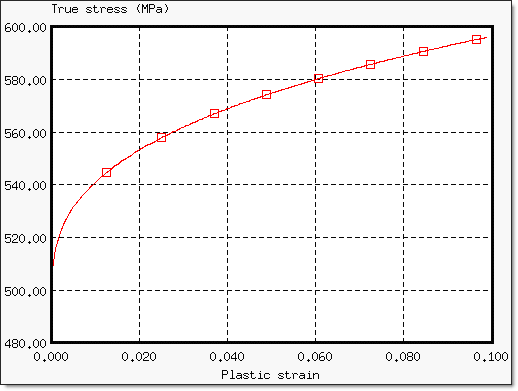
Figure 6. Yield Curve of the Johnson-Cook Model:
- Material Properties
- Young's modulus
- 73000
- Poisson's ratio
- 0.33
- Density
- 0.0028
- Material Properties
- Young's modulus
- 210000
- Poisson's ratio
- 0.33
- Density
- 0.0078
- Bars
- Length
- 4 m
- Diameter
- 12 mm
- Projectile
- Radius
- 12 mm
- Weight
- 170 g
High Strain Rate Test Method
- Modulus of the output bar,
- Strain associated with the output stress wave
- Cross-section of the output bar
If the two bars remain elastic and wave dispersion is ignored, then the measured stress pulses can be assumed to be the same as those acting on the object.
- and
- Strains associated with input stress wave
- Strain associated with output stress wave
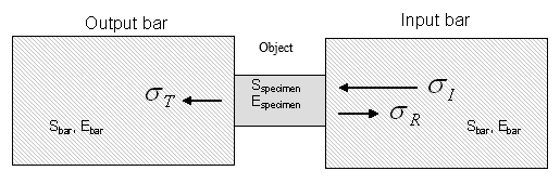
Figure 7. 1D Analysis
- Interface 1
- Interface 2
- Balance in object
- Engineering stress in object
Model Method
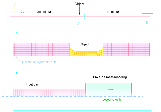
Figure 8. Axisymmetrical Model Mesh with Imposed Velocities on the Top of the Input Bar
Strain Rate Filtering
Because of the dynamic load, strain rates cause high frequency vibrations which are not physical. Thus, the stress-strain curve may appear noisy. The strain rate filtering option enables to dampen such oscillations by removing the high frequency vibrations in order to obtain smooth results. A cut-off frequency for strain rate filtering, Fcut = 30 kHz was used in this example. Good engineering judgment should be used to determine a good value for each simulation. Refer to Example 11 - Tensile Test for further details.
Results
The purpose of this test is to obtain the results observed in experiments with a Johnson-Cook model. The increase of stress is expected to equal approximately 30% compared to the low strain rate test.
Experimental Data
Experimental results show that the variation of the true tensile flow stress compared with the true strain is approximately equivalent to a strain rate between 80 s-1 and 100 s-1. The reference strain, in the Johnson-Cook model is set to 0.08 ms-1. At higher rates, the true flow stress increases significantly compared with the strain rate. The 7010 aluminum alloy exhibits an increase in the flow stress by a typical 30% at high strain rates (900 s-1 to 3000 s-1) compared to static values.
Results are given at the specific true strains of 0.02, 0.05 and 0.10. The influence of the strain rate on stress can be seen in Figure 9 1:
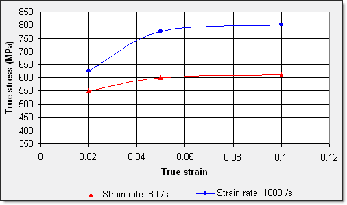
Figure 9. Variation of True Stress Compared with True Strain for 7010 Alloy using 2 Different Rates (experimental data)
| Strain rate: 80 s-1 | Strain rate: 900 s-1 | ||||||
|---|---|---|---|---|---|---|---|
| True strain | 0.02 | 0.05 | 0.1 | 0.02 | 0.05 | 0.1 | 0.25 |
| True stress (MPa) | 550 | 600 | 610 | 625 | 775 | 800 | 850 |
Johnson-Cook Model
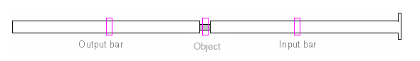
Figure 10. Stress Measurement Localizations
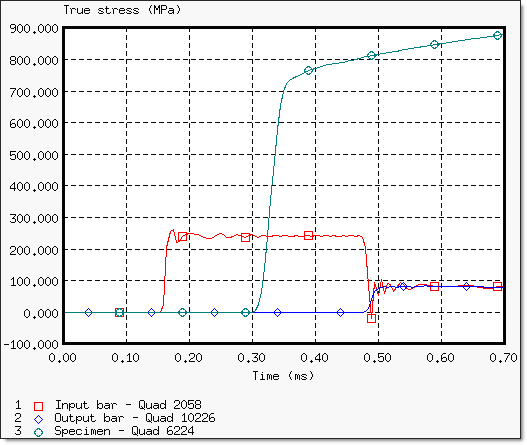
Figure 11. Stress Waves in the Input Bar, the Output Bar and the Object (imposed velocities = 5.8 ms-1 )
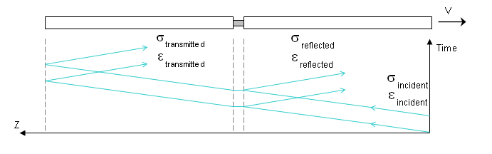
Figure 12. SHPB of the Motion in Time of the Tensile Pulse
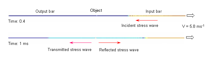
Figure 13. von Mises Stress Wave Propagation Along Bars (imposed velocities = 5.8 ms-1 )
- 5189 ms-1
- Young's modulus
- Density of the bars
The time step element is controlled by the smallest element located in the object. It is set at 5x10⁻⁵ ms. The stress wave thus reaches the object in 0.77 ms and travels 0.26 mm along the bar for each time step. Obviously, it remains lower than the element length of the smallest dimension (0.88 mm).
An imposed velocity of 5.8 ms-1 produces a strain rate in the object of approximately 900 s-1, while a strain rate of approximately 80 s-1 is achieved using an imposed velocity of 1.7 ms-1. A simulation is performed for each velocity value. It should be noted that the study on low rates is more limited in time than on high rates due to the reflected wave generated on top of the output bar.
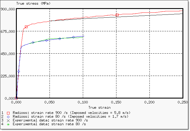
Figure 14. Variation of True Stress with True Strain for High and Medium Strain Rates
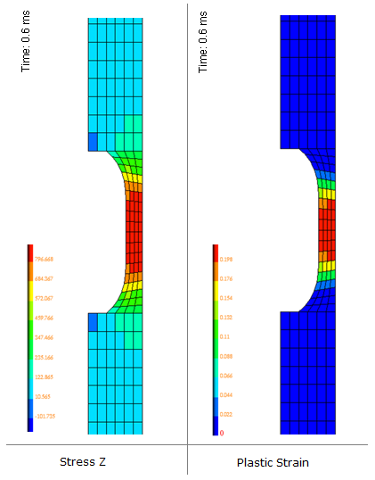
Figure 15. Stress Z and Plastic Strain on Object at 0.6 ms
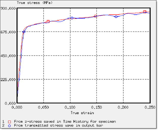
Figure 16. True Stress Comparison in the Object
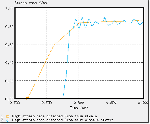
Figure 17. True Strain Rate in the Object (using both computations)
Either data sources used to evaluate the strain rate give similar results.
- the strain rate effect on stress, with or without the cut-off frequency for smoothing (100 kHz);
- the influence of the strain rate coefficient (comparison with experimental data).
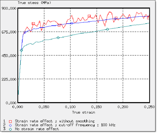
Figure 18. Strain Rate Effect
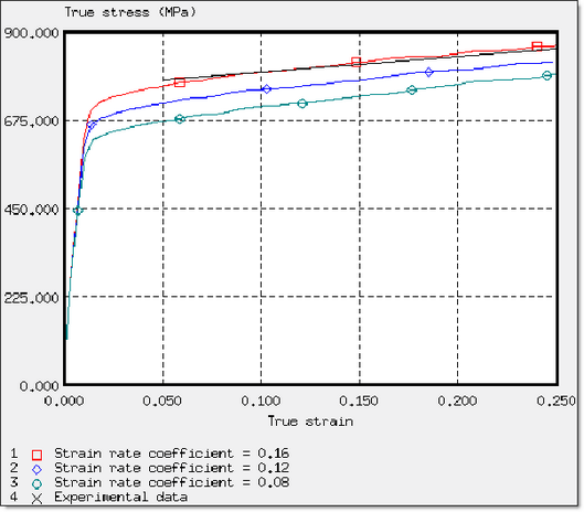
Figure 19. Influence of the Strain Rate Coefficient c
These studies are performed for the high strain rate model ( = 900 s-1).
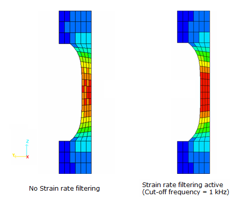
Figure 20. Comparison of the Distribution of the von Mises Stress at Time t=0.6 ms
More physical flow stress distribution is obtained using filtering. Explicit is an element-by-element method, while the local treatment of temporal oscillations puts spatial oscillations into the mesh.