RD-E: 2400 Laminating
Two rolling rigid cylinders squeeze a plate to laminate it.
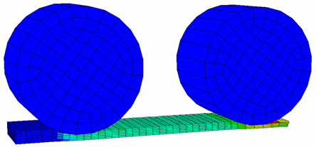
Figure 1.
Options and Keywords Used
- Brick element, solid formulation, co-rotational formulation, and fully-integrated element
- Constant pressure formulation and plasticity options
- Large deformation / Small strain
- Interface (/INTER/TYPE7)
Contact between the metal strip and the rollers are modeled by a TYPE7 interface. The main surface is defined by the external surface of the rollers, and the secondary nodes by the metal strip (/GRNOD/PART). As there is only one element over the width of the rollers. The previous interface does not need to be symmetrically arranged. The gap is chosen arbitrarily at 1 mm.
- Boundary conditions (/BCS)
The lower nodes of the metal strip are constrained in Z (to represent the moving machine bed).
The main nodes of the rollers are constrained in all directions, except rotation around the X-axis.
- Constant time step (/DT/BRICK/CST)
- Imposed velocities (/IMPVEL)
A constant angular velocity around the X-axis is applied to both of the rollers' main nodes.
- Initial velocity (/INIVOL)
An initial velocity of 500 mm/s in the X-direction is applied to every node of the metal strip.
- Elasto-plastic material law (/MAT/LAW2 (PLAS_JOHNS))
- General solid property (/PROP/TYPE14 (SOLID))
- Rigid body (/RBODY)
Input Files
- Thickness:
- 2 elements
- <install_directory>/hwsolvers/demos/radioss/example/24_Laminating/Thickness/2_elements/ROLLING*
- 5 elements
- //.../24_Laminating/Thickness/5_elements/ROLLING*
- Formulation:
- Isolid=17
- <install_directory>/hwsolvers/demos/radioss/example/24_Laminating/Formulation/Isolid17/ROLLING*
- Icpre=0
- //.../24_Laminating/Formulation/Icpre0/ROLLING*
- Icpre=1
- //.../24_Laminating/Formulation/Icpre1/ROLLING*
- Temperature:
- T=800°C
- <install_directory>/hwsolvers/demos/radioss/example/24_Laminating/temperature/T=800/ROLLING*
- T=1200°C
- //.../24_Laminating/temperature/T=1200/ROLLING*
Model Description
Units: mm, s, Mg, N, MPa
This analysis shows a phase of a rail rolling. A metal strip is successively passed through two rollers aiming at reducing its thickness. Both rollers have a constant angular velocity of 6.85 rad/s, and the metal strip is dragged along a moving machine bed. This process may be considered quasi-static and involves high deformation (mainly compression).
- Material Properties
- Initial density
- 7.8 x 10⁹ Mg/mm3
- Young's modulus
- 210000
- Poisson ratio
- 0.3
- Yield stress
- 170
- Hardening parameter
- 400
- Hardening exponent
- 0.475
- Parameters
- Temperature exponent
- 1
- Melting temperature
- 2073 K (around 1800°C)
- Specific heat at constant pressure Cp
- 460
- Geometry
- The metal strip has a cross-section of 80 x 20 mm and the rollers have a radius of 100 mm. After the passage of the first roller, the thickness is reduced by 7 mm, then by another 5 mm after the second roller.
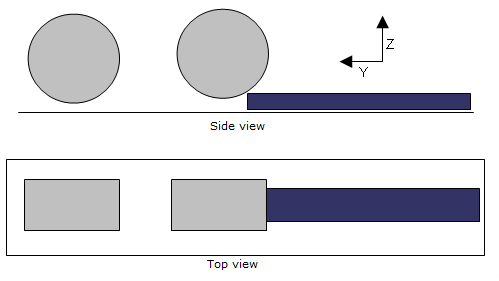
Figure 2. Geometry of the Problem
Model Method
It is not necessary to pass many elements over the width of the metal strip, but rather to obtain an accurate stress distribution over its thickness by passing a minimum of five elements over the thickness of the metal strip. Depending on what is being looked for, passing five elements over the thickness may seem like a lot. This issue should be discussed in the early part of the analysis. Concerning the rollers as the elements is of first order, as it is not easy to perfectly model the curvature. The mesh must be fine enough to estimate the curvature with as much accuracy as possible, one element over the width being sufficient.
Some details are made: The moving machine bed is not modeled and all lower nodes of the metal strip are constrained in the Z-direction. Moreover, an initial velocity is applied to the metal strip to initiate contact with the first roller. Assuming there is a Coulomb friction between the metal strip and the roller using a friction coefficient of 0.3, the metal strip is then dragged by the roller.
Assuming the rollers are rigid, a constant angular velocity to the main nodes is applied.
Results
Number of Elements over the Thickness
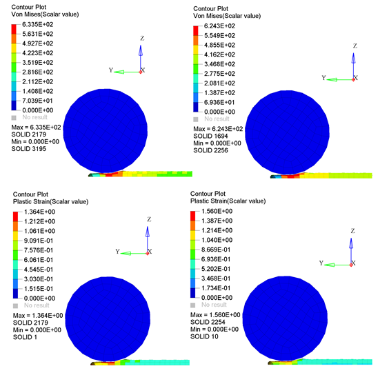
Figure 3. Comparison Between Two and Five Elements
Passing two elements over the thickness is not enough to see the stress (or strain) distribution; five elements is enough though. If the deformed shape is not smooth and/or the gradient between the two elements is too high, consider refining the mesh; however, this can be somewhat costly! Additionally, it takes 12 times longer to run the model with five elements over the width.
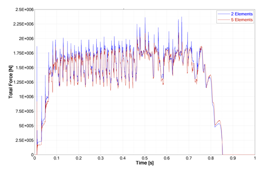
Figure 4. Reaction Forces Acting on the Cylinder
The above graph indicates the reaction force on the first cylinder using two or five elements over the thickness. Both curves are almost identical and it takes much longer to use five elements. Thus, to save CPU time, there is no need to use more than two elements.
Small Strain Formulation Influence
Usually for problems involving large deformations, a large strain formulation would be used. In Radioss this is the default setting, but it is also possible to use a small strain formulation. This formulation is not very accurate for large deformations, but it is more robust and enables the time step to not decrease too much. Indeed, large deformation/rotation problems may lead to mesh distortion which causes the time step to drop drastically; computation may even stop due to a negative volume. The small strain formulation overcomes all this by assuming a constant volume, consequently the time step becomes constant, and even if the mesh is completely distorted, computation will not be stopped due to the negative volume.
This formulation can be applied from t=0 by setting the flag Ismstr to 1, directly in the type of a specific part. It is also possible to switch from a large strain formulation to a small strain formulation during the simulation in order to prevent a negative volume and/or to maintain a decent time step using the /DT/BRICK/CST option in the Engine file (*_0001.rad) having a critical time step.
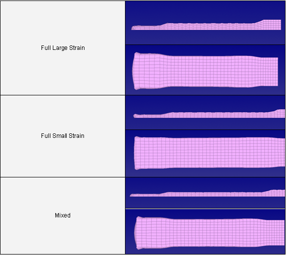
Figure 5. Deformed Shape
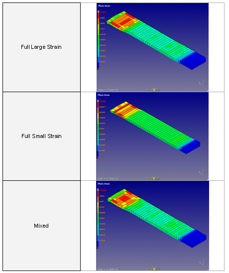
Figure 6. Deformed Shape
In such a case, it may be of interest to use the small strain formulation but only for a few elements reaching a critical time step (using /DT/NODA/CST); as the time step will not stop, due to a distorted element. However, for accuracy reasons, the number of elements switching to a small strain formulation should be checked, the lower the better.
HA8 Formulation Influence
The improved solid formulation HA8 overcomes the drawbacks of the standard 8 integration points' formulation (Isolid=17 or 14). In particular, in the case of a pure bend, "shear-locking", which makes the standard formulation rather stiffer, does not exist. It is also possible to use the small strain formulation, which contrary to the 8 integration points' formulation is not compatible. It is now possible to use up to 9 integration points for each direction.
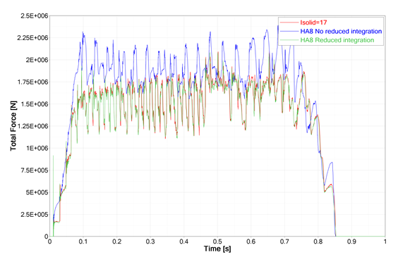
Figure 7. Rolling Force for Different Formulations
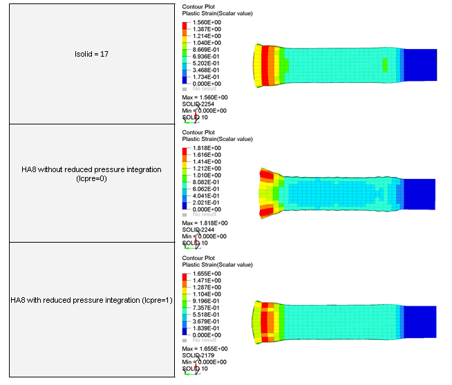
Figure 8. Plastic Strain for Different Formulations
The HA8 formulation must always be used with reduced pressure integration, the only time when this option must be deactivated is in the case of emulating a thick shell formulation with 8-nodes bricks.
Temperature Influence
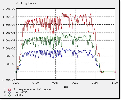
Figure 9. Rolling Force
Conclusion
The squeezing of the metal strip below two rolling cylinders is simulated by Radioss. The large deformation formulation, when a sufficient number of elements are used, obtaining physically-acceptable results is allowed. The small strain option leads to bad results, but with low cost. The element formulation and the number of integration points through thickness are other parameters influencing results; the higher the precision, the higher the cost. On the other hand, as the problem is considered to be quasi-static, resolution using the Radioss implicit solver can be envisaged.