RD-E: 2500 Spring-back
An explicit stamping simulation is followed by a spring-back analysis using implicit or explicit solvers for stress relaxation.
The spring-back simulation of sheet metal bent into a hat-shape is studied. The problem is one of the famous tests from the Numisheet'93. As spring-back is generally a quasi-static unloading, the use of the Radioss implicit solver is justified. The Radioss explicit solver is also used to compare the method's efficiency. However, for the stamping phase only the explicit solver is used, as the forming process is highly dynamic.
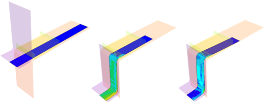
Figure 1.
Options and Keywords Used
- Explicit stamping simulation, implicit / explicit spring-back simulation, and stress relaxation
- Implicit strategy and time step control by arc-length method
- Anisotropic elasto-plastic material law (/MAT/LAW43 (HILL_TAB)) and Hill model
- Orthotropic shell formulation, QEPH, progressive plastification, and iterative plasticity
- Interface (/INTER/TYPE7), Penalty method, and friction
- Concentrated load (/CLOAD)
- Dynamic relaxation (/DYREL)
- Implicit parameters (Implicit Solution)
- Implicit spring-back (/IMPL/SPRBACK)
- Imposed velocity (/IMPVEL)
- Rigid body (/RBODY)
- Stamping simulation by explicit: from the beginning up to 960 ms.
- Spring-back simulation:
- using explicit (dynamic approach): from 960 ms to 6000 ms:
- From 960 ms to 2000 ms: Stamping tools are slowly withdrawn because the quasi-static analysis requires dynamic effects to be minimized during spring-back. Thus, the interfaces are not deleted. Options are defined in the *_0002.rad Engine file.
- From 2000 ms to 6000 ms: A dynamic relaxation (/DYREL) is activated in the *_0003.rad Engine file in order to converge towards quasi-static equilibrium.
- using implicit (static approach): from 960 ms to 1000 ms:
- The input implicit options are added in the *_0002.rad Engine file. Stress relaxation is activated using the /IMPL/SPRBACK keyword. All interfaces are deleted and specific boundary conditions are added on the stamping tools. Tools are not withdrawn.
- using explicit (dynamic approach): from 960 ms to 6000 ms:
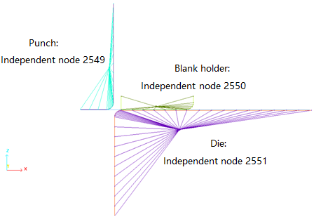
Figure 2. Modeling of the Stamping Tools as Rigid Elements
An automatic main node is chosen. The center of gravity is computed using the main and secondary node coordinates and the main node is moved to the center of gravity where is placed mass and inertia (ICoG is set to 1). No mass or inertia are added to the rigid bodies.
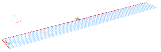
Figure 3. Boundary Conditions (/BCS) on the Sheet Metal According to the Symmetries
The nodes on the longitudinal plane are fixed in the Y translation and X, Z rotations.
For the other symmetry plane, the nodes are fixed in the X translation and Y, Z rotations.
Stamping tools are restricted to moving only along the Z-axis. The boundary conditions are applied on the main nodes of the rigid bodies, including the parts (Figure 3).
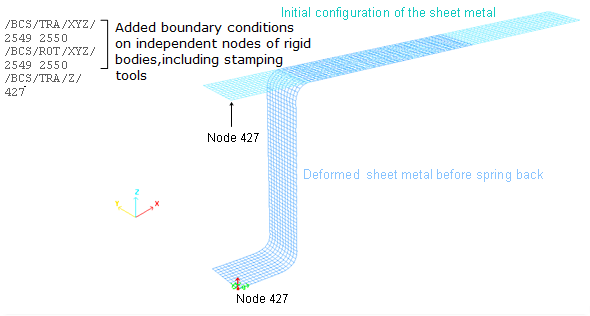
Figure 4. Added Boundary Conditions on the 427 Node for Implicit Spring-back
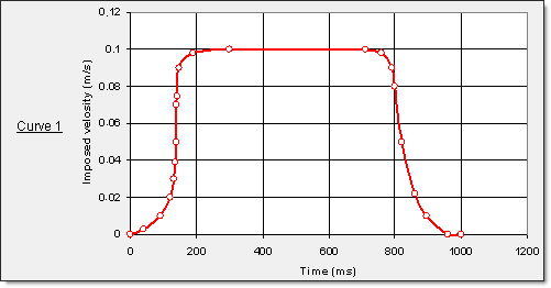
Figure 5. Imposed Velocity on Punch via the Rigid Body's Main Node
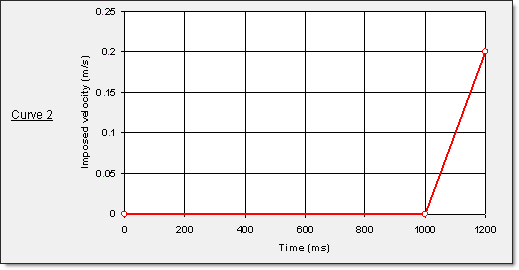
Figure 6. Imposed Velocity on Die and Blank Holder via the Rigid Bodies' Main Node
" Punch part …………… Curve 1, scale factor set to -1.
" Die part …………… . Curve 2, scale factor set to 1.
" Blank holder part ……. Curve 2, scale factor set to -1.
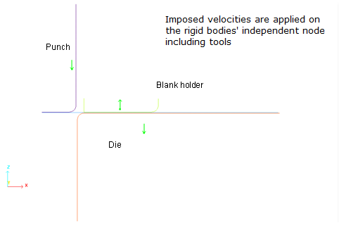
Figure 7. Imposed Velocities on Tools in Two Phases: Stamping then Tools Removing
Considering the symmetries, a constant concentrated load of 612.5 N is vertically applied on the blank holder via the main node of the rigid body. The load is set to zero from 960 ms before studying the spring-back.
Implicit spring-back analysis is launched using /IMPL/SPRBACK.
A solver method is required to resolve Ax=b in each iteration of the nonlinear cycle. It is defined using /IMPL/SOLVER.
|
|
|
|
|
|
|
|
|
|
Refer to Radioss Starter Input for more details about implicit options.
|
|
Refer to Radioss Starter Input for more details about implicit options.
Explicit spring-back analysis uses the dynamic relaxation in the *_0003.rad Engine file from 2000 ms.
The explicit time integration scheme starts with nodal acceleration computation. It is efficient for the simulation of dynamic loading. However, a quasi-static simulation via a dynamic resolution method is needed to minimize the dynamic effects for converging towards static equilibrium, the final shape achieved after spring-back.
- Relaxation value which has a recommended default value
- Period to be damped (less than or equal to the highest period of the system)
- Relaxation factor
- 1
- Period to be damped
- 1000 ms
This option is activated using the /DYREL keyword (inputs: and ).
Input Files
- Explicit spring-back
- <install_directory>/hwsolvers/demos/radioss/example/25_Spring-back/Explicit_spring-back/DBEND_44*
- Implicit spring-back
- <install_directory>/hwsolvers/demos/radioss/example/25_Spring-back/Implicit_spring-back/DBEND_44*
Model Description
This example deals with the numerical simulation of a stamping process, including the spring-back.
This refers to one of the sheet metal stamping tests "2D Draw Bending" indicated in Numisheet’93. The final shape of the formed sheet metal, after releasing all constraints on the blank sheet is studied. During the spring-back simulation, an explicit-to-implicit sequential solution method is used, where a dynamic forming process using the explicit solver is used first, followed by an implicit modeling of the spring-back deformations by statically removing the stamping stress.
- Explicit stamping and implicit spring-back simulations
- Explicit stamping and explicit spring-back simulations (using dynamic relaxation)
The spring-back simulation of the forming sheet metal uses an elasto-plastic nonlinear approach. The implicit input options and the incremental strategy used are described in the modeling section.
A numerical simulation of stamping is performed up to 960 ms. Spring-back computation is carried out from 960 ms to 1000 ms for implicit (static approach) and to 6000 ms for explicit (quasi-static approach).
A standard stamping operation is studied. The stamping tools include a punch, a die and a blank holder.
Units: mm, ms, g, N, MPa.
A load F of 1225 N is vertically applied on the blank holder in order to flatten the sheet metal against the die. The load is removed before spring-back simulation.
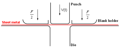
Figure 8. Description of the Problem
- Radius of die's corners
- 5 mm
- Radius of punch's corners
- 5 mm
- Width of punch
- 50.4 mm
- Sheet metal dimensions
- 35 mm x 175 mm
The thickness of the sheet metal is defined at 0.74 mm. The Coulomb friction coefficient between the sheet metal and the die is defined at 0.129.
- Material Properties
- Initial density
- 8x10⁻³
Note: The density is artificially increased from 8x10⁻³ to minimize the run time.
- Young's modulus
- 206000
- Poisson ratio
- 0.3
The material of the sheet metal under the roller has distinct characteristics of anisotropy. Its anisotropic elasto-plastic behavior can be reproduced by a Hill model (/MAT/LAW43). This law can be considered as a generalization of the von Mises yield criteria for anisotropic yield behavior.
The coefficients are determined using Lankford's anisotropy parameters range. Angles for Lankford parameters are defined with respect to orthotropic direction 1.
- Material Properties
- Initial density
- 8x10⁻³
- Young's modulus
- 206000
- Poisson ratio
- 0.3
- Lankford 0 degrees
- r00= 1.73
- Lankford 45 degrees
- r45 = 1.34
- Lankford 90 degrees
- r90= 2.24
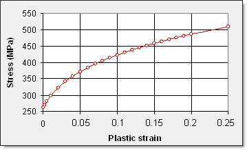
Figure 9. User's Yield Function
Model Method
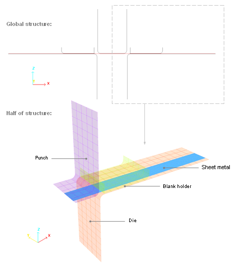
Figure 10. Finite Mesh Elements of the Problem Studied
The punch is shown in purple, the blank holder in green and the die in red. The sheet metal (blue) is modeled using 4-node shell elements.
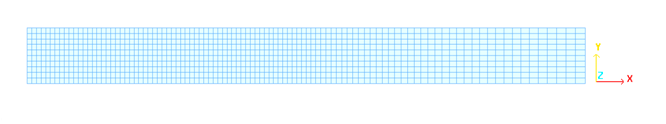
Figure 11. Progressive Mesh of the Sheet Metal
In order to achieve accurate simulation results, the QEPH shell element formulation is used in explicit and implicit analyses. A Lagrangian formulation is adopted.
- Five integration points (progressive plastification)
- Interactive plasticity with three Newton iterations (Iplas = 1)
- Thickness changes are taken into account in stress computation (Ithick = 1)
- Initial thickness is uniform, equal to 0.74 mm
- Orthotropy angle: 0 degree
- Reference vector: (1 0 0)
The input components of the reference vector are used to define direction 1 of the local coordinate system of orthotropy. The orthotropy angle, in degrees defines the angle between direction 1 of the orthotropy and the projection of the vector on the shell.
- Material Properties
- Coulomb friction
- 0.129
- Gapmin
- 0.37
- Critical damping coefficient on interface stiffness
- 1
- Critical damping coefficient on interface friction
- 1 (default)
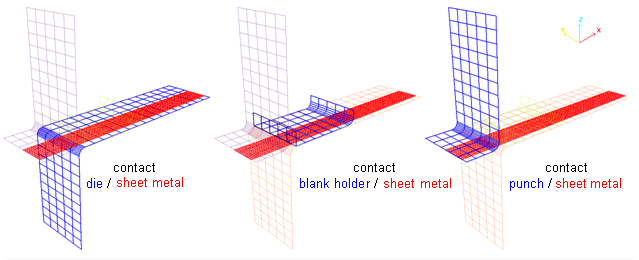
Figure 12. Contact Modeling using a TYPE7 Interface Considered with the Penalty Method (main/secondary sides)
In the implicit approach, the contact using the Penalty method with fictional springs is stored in a separate stiffness matrix to the main one. Therefore, supplementary memory is needed and information of the second contact stiffness will be printed when contact is active.
- The normal force computation is indicated by:
(4) 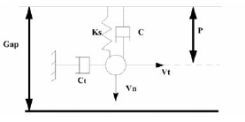
Figure 13.Where,- Initial interface spring stiffness
- Critical damping coefficient on interface stiffness (default value: 0.05)
- The tangential force computation is indicated by:
(5) Where,- Critical damping coefficient on interface friction (default value: 1)
For spring-back computation by implicit, the removing of the stamping tools is taken into account by deleting all interfaces using the input option in the second *_0002.rad Engine file as:/DEL/INTER 1 2 3Interfaces ID 1, 2 and 3 are deleted.
Results
In the metal stamping operation, the highly nonlinear deformation processes tend to generate a large amount of elastic strain energy in the metal material in addition to some of the plastic deformed areas. The internal energy, which is stored in the sheet metal during stamping, is subsequently released once the stamping pressure has been removed. This energy released is the driving force of the spring-back in the sheet metal forming process. Therefore, the spring-back deformation for sheet metal forming is mainly due to the amount of elastic energy stored in the part while it is being plastically deformed.
The material density has been multiplied by 10,000 to obtain a reasonable computation time using explicit simulations. An additional time period is also required for slowly withdrawing the tools, prior to the explicit spring-back simulation in order to achieve a good result. Thus, explicit stamping takes longer than stamping followed by implicit spring-back computation.
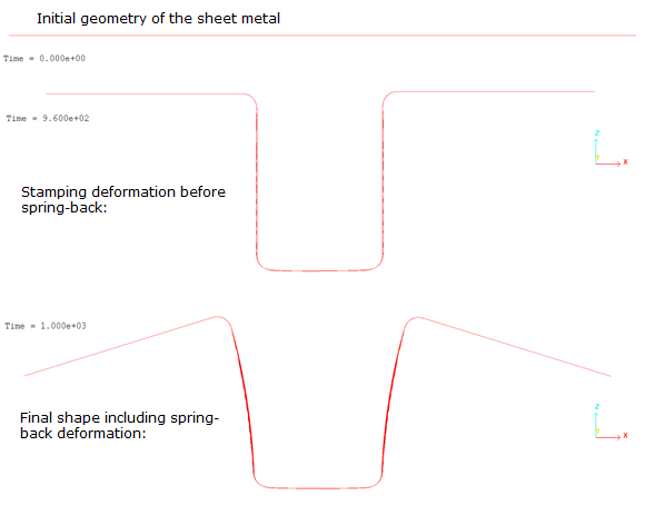
Figure 14. Deformed Sheet Metal Before and After Spring-back (implicit spring-back)
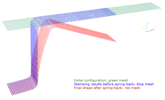
Figure 15. Deformed Mesh of the Sheet Metal Before and After the Spring-back (multi-models mode)
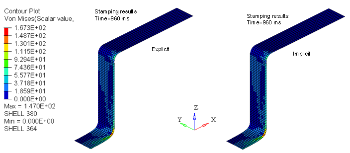
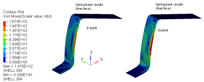
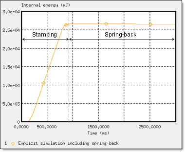
Figure 17. Internal Energy in the Sheet Metal Part (explicit spring-back simulation)
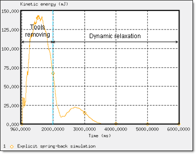
Figure 18. Convergence Towards Quasi-static Equilibrium (explicit spring-back simulation)
| 1 | 2 | |
|---|---|---|
| Experiment (means values) | 105.7 | 77.7 |
| Implicit | 100.8 | 78.6 |
| Explicit | 106.1 | 78 |
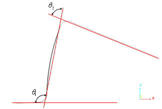
Figure 19.
| Stamping CPU (cycles) | Spring-back
Cycles (iter. Num.) |
Spring-back
CPU (CPU per cycle) |
Total CPU | |
|---|---|---|---|---|
| Explicit | 1160 (92326) | 229379 (-) | 2698 (0.01) | 3858 |
| Implicit | - | 120 (354) | 1589 (13.2) | 2749 |
The implicit simulation for spring-back is performed from 960 ms to 1000 ms. Explicit spring-back simulation is performed until the kinetics energy on the sheet metal reaches a minimum value (quasi-static equilibrium). The final computation time is set to 6000 ms.
Explicit and implicit analysis' both obtain good results in this test, with implicit computation being 40% faster than the explicit computation. The implicit approach is; however, 1320 times more expensive per step than the explicit solver. The use of the implicit approach allows you to economize on the overall computation time.