RD-E: 1900 Wave Propagation

Elastic wave propagation on a half-space subjected to a vertically-distributed load.

Elastic shock wave propagation on a half-space is studied using two different approaches:
  • Lagrangian formulation
  • ALE (Arbitrary Lagrangian Eulerian) formulation.
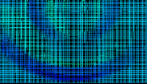
The simulation results are compared with an analytical solution. A bi-dimensional problem is considered.

rad_ex_19_wave
Figure 1.

The domain subjected to the vertical impulse load undergoes an elastic material law process. The generated shock wave is composed of a longitudinal wave and a shear wave. Results are indicated in 0.77 ms, for which the longitudinal wave is predicted to reach the lower boundary of the domain. In order to ensure an accurate wave expansion, an infinite domain is modeled using a non-reflective frontiers (NRF) material law available in the ALE formulation.

Options and Keywords Used

  • Bi-dimensional analysis (/ANALY), quad and general solid

    A bi-dimensional problem is considered. The flag N2D3D defined in /ANALY is set to 2. The 2D analysis defines the X-axis as the plane strain direction.

  • Impulse load, shock wave propagation, longitudinal and shear waves
  • ALE and Lagrangian modeling
  • Non-reflective frontiers (NRF) material and infinite domain
  • ALE material formulation (/ALE/MAT)
  • Concentrated load (/CLOAD)
    The applied vertical pulse is a concentrated load (/CLOAD) in the form of a sinusoidal function having an amplitude F = 1 MathType@MTEF@5@5@+= feaagKart1ev2aaatCvAUfeBSjuyZL2yd9gzLbvyNv2CaerbwvMCKf MBHbqefqvATv2CG4uz3bIuV1wyUbqedmvETj2BSbqefm0B1jxALjhi ov2DaebbnrfifHhDYfgasaacH8srps0lbbf9q8WrFfeuY=Hhbbf9v8 qqaqFr0xc9pk0xbba9q8WqFfea0=yr0RYxir=Jbba9q8aq0=yq=He9 q8qqQ8frFve9Fve9Ff0dmeaacaGacmGadaWaaiqacaabaiaafaaake aacaWGgbGaeyypa0JaaGymaaaa@3B63@ GPa and a time period of T = 2 π E 5 s MathType@MTEF@5@5@+= feaagKart1ev2aaatCvAUfeBSjuyZL2yd9gzLbvyNv2CaerbwvMCKf MBHbqefqvATv2CG4uz3bIuV1wyUbqedmvETj2BSbqefm0B1jxALjhi ov2DaebbnrfifHhDYfgasaacH8srps0lbbf9q8WrFfeuY=Hhbbf9v8 qqaqFr0xc9pk0xbba9q8WqFfea0=yr0RYxir=Jbba9q8aq0=yq=He9 q8qqQ8frFve9Fve9Ff0dmeaacaGacmGadaWaaiqacaabaiaafaaake aacaWGubGaeyypa0JaaGOmaiabec8aWjabgEHiQiaadweadaahaaWc beqaaiabgkHiTiaaiwdaaaGccaWGZbaaaa@41C3@ .

    rad_ex_fig_19-4a
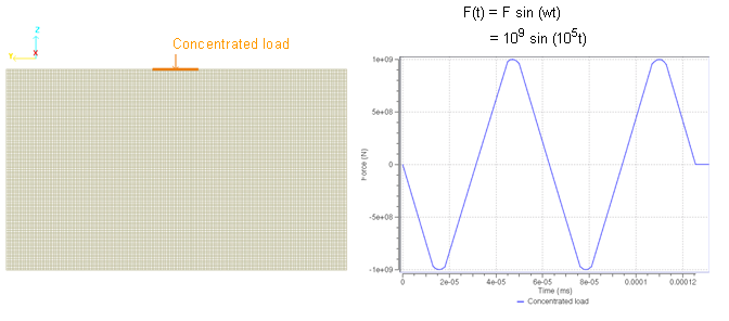
    Figure 2. Variation of the Impulse Load Over Time
  • Function (/FUNCT)
  • Non-reflective frontiers (NRF) material LAW11 (/MAT/LAW11 (BOUND))
Lagrangian Modeling Specific Options
Boundary conditions: Three sides of the model are fixed in terms of translation.

rad_ex_fig_19-5
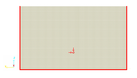
Figure 3. Fixed Sides

The limitation of this approach is the reflection on the domain's boundaries. Simulation results are shown for the point in time prior to the shock hitting the low side (< 0.77 ms).

ALE Modeling Specific Options
Non-reflective frontiers (NRF): The mesh includes quiet boundary elements to model the infinite domain. These elements minimize the reflection of the propagating waves. The material used for these elements follow a non-reflective frontiers (NRF) material LAW11 (TYPE3) as a non-reflective frontiers (NRF), with the following characteristics:
Material Properties
Initial density
2842 kg.m3
Characteristic length
0.0632m

rad_ex_fig_19-6
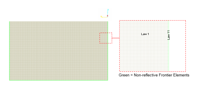
Figure 4. Infinite Domain Modeled by the Non-reflective Frontiers (NRF) Material LAW11 (TYPE3)

The materials have to be declared ALE using /ALE/MAT in the input desk.

Input Files

The input files used in this example include:
Lagrangian modeling
<install_directory>/hwsolvers/demos/radioss/example/19_Wave_propagation/Lagrangian_formulation/WAVE*
ALE modeling
<install_directory>/hwsolvers/demos/radioss/example/19_Wave_propagation/ALE_formulation/WAVE*

Model Description

Units: m, s, Kg, N, Pa.

A half-space is subjected to a vertical load distributed over a varied time span and creating wave propagation in the domain. The dimensions of the model are 8 m x 4.76 m and the impulse load is applied over a 1 m-width zone.

rad_ex_fig_19-1
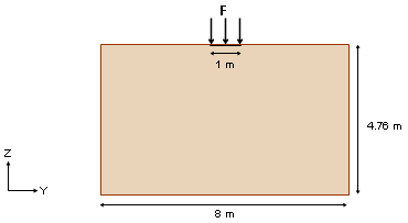
Figure 5. Problem Data
The material used follows a linear elastic law (/MAT/LAW1) with the following characteristics:
Material Properties
Initial density
2842 kg.m-3
Young's modulus
73 GPa
Poisson ratio
0.33

The expansion process of the shock wave is comprised of the longitudinal and shear waves.

Based on these material properties, the propagation speed of longitudinal waves in the material correspond to 6169.1 m.s-1 and 3107.5 m.s-1 for shear waves. Thus, the longitudinal waves should reach the lower boundary of the domain in about 0.77 ms.

The wave pattern caused by a distributed load is shown in Figure 6.

rad_ex_fig_19-2
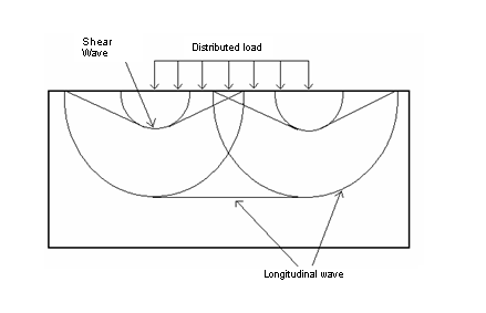
Figure 6. Longitudinal and Shear Waves Comprising the Wave Pattern

The impulse load is described by the sinusoidal function: F ( t ) = sin ( 2 10 5 t ) G P a MathType@MTEF@5@5@+= feaagKart1ev2aaatCvAUfeBSjuyZL2yd9gzLbvyNv2CaerbwvMCKf MBHbqefqvATv2CG4uz3bIuV1wyUbqedmvETj2BSbqefm0B1jxALjhi ov2DaebbnrfifHhDYfgasaacH8srps0lbbf9q8WrFfeuY=Hhbbf9v8 qqaqFr0xc9pk0xbba9q8WqFfea0=yr0RYxir=Jbba9q8aq0=yq=He9 q8qqQ8frFve9Fve9Ff0dmeaacaGacmGadaWaaiqacaabaiaafaaake aacaWGgbWaaeWaaeaacaWG0baacaGLOaGaayzkaaGaeyypa0Jaci4C aiaacMgacaGGUbWaaeWaaeaacaaIYaGaey4fIOIaaGymaiaaicdada ahaaWcbeqaaiaaiwdaaaGccaWG0baacaGLOaGaayzkaaGaaGjbVlaa dEeacaWGqbGaamyyaaaa@4AAE@

Model Method

The part is modeled using a regular mesh with 19080 QUAD elements (44.9 mm x 44.4 mm with l c =63.15 mm).


rad_ex_fig_19-3
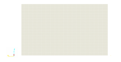
Figure 7. Mesh of the Bi-dimensional Domain

Results

Comparison of Lagrangian and ALE Results with the Analytical Solution

Figure 8 and Figure 9 represent the von Mises stress wave propagation and the velocities at t=0.77 ms.

rad_ex_fig_19-7
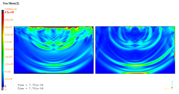
Figure 8. von Mises isovalues at t=0.77 ms

rad_ex_fig_19-8
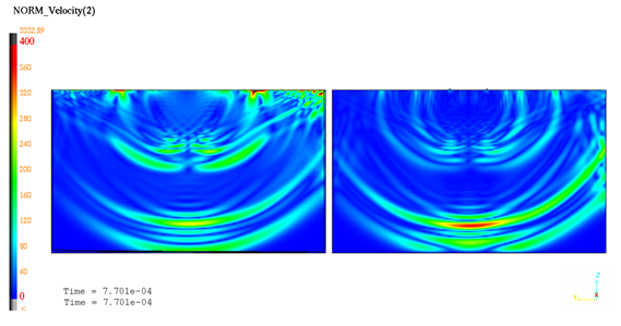
Figure 9. Velocity isovalues at t=0.77 ms

The shock wave propagation is well predicted. Simulation results obtained at t=0.77ms corroborate the analytical solution: Longitudinal and shear waves.

Lagrangian Results

Wave Pattern

The wave pattern produced by the distributed load shown previously can be identified in the deformed configuration when the longitudinal wave reaches the lower boundary of the mesh.

rad_ex_fig_19-9
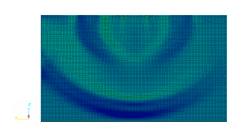
Figure 10. Wave Pattern in Domain at t=0.77 ms

Vertical Displacement

The graphs below show the vertical displacement (DZ) of three nodes respectively positioned at 0 m, 3.2 m and 4.75 m under the edge of the distributed load.

rad_ex_fig_19-10
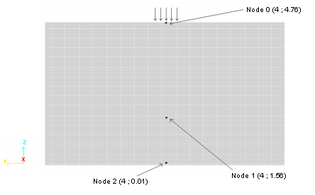
Figure 11. Nodes Saved in Time History
Figure 12 shows the vertical displacement of Node 0. The beginning of the wave propagation can be seen during the time [0; 1.35e-04]. The response after the end of the application force [1.35e-04; 4e-04] is due to the shear wave.

rad_ex_fig_19-11
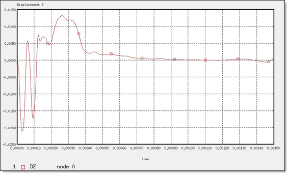
Figure 12. Z-displacement of "Node 0"
The vertical response of Node 1 shows that the longitudinal wave reaches it in 0.47 ms (Figure 13). The reflection can be seen after 0.97 ms. The shear wave does not appear because its motion is in the horizontal direction.

rad_ex_fig_19-12
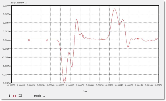
Figure 13. Z-displacement of "Node 1"
The displacement of Node 2 placed at the other extremity of the pattern, shows that the longitudinal wave crosses the model in 0.7 ms, in accordance with the analytical results.

rad_ex_fig_19-13
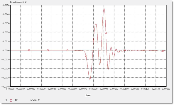
Figure 14. Z-displacement of "node 2"

Horizontal Displacement

Figure 15 shows the horizontal displacement of Node 1 (placed 3.2 m below the load surface). The horizontal component of the longitudinal wave reaches the node in 0.49 ms, while the shear wave arrives at 1.1 ms. Any response after this time results from the different reflections of the longitudinal and shear waves.

rad_ex_fig_19-14
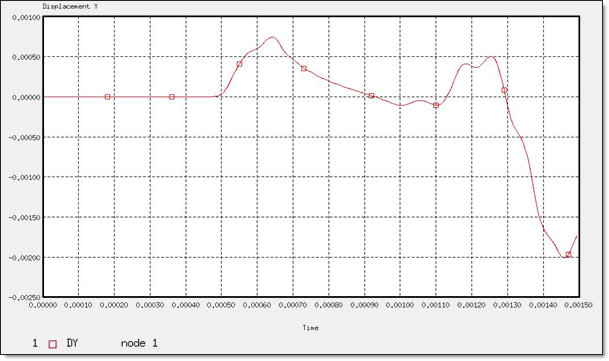
Figure 15. Y-displacement of "node 0"

rad_ex_fig_19-15
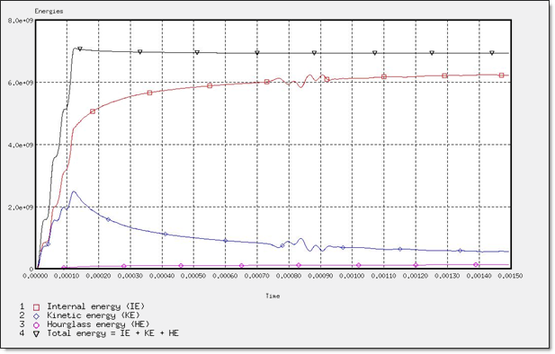
Figure 16. Global Energy Assessment

ALE Results

The wave pattern produced by a distributed load can be identified in the deformed configuration by displaying the pressure. The grid is fixed and nodal displacements are equal to zero. Figure 17 shows propagation when the longitudinal wave reaches the lower boundary of the mesh.

rad_ex_fig_19-16
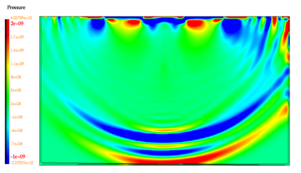
Figure 17. Pressure isovalues at time t=0.77 ms

Conclusion

The wave propagation in a finite domain is studied using Lagrangian and ALE approaches. The Lagrangian formulation does not allow an infinite domain to be defined. Reflections of the longitudinal and shear waves against boundaries restrict simulation in terms of time (t < 0.77 ms). The ALE approach allows you to model an infinite domain by defining the non-reflective frontiers (NRF) material (LAW11 - TYPE3) on the limits. Such specific modeling minimizes the reflection of the expansion wave.

The bi-dimensional analysis illustrates a planar propagation. An accurate representation of the wave pattern is obtained and the simulation results are in a closed agreement with the analytical solution.