RD-E: 1803 Square Membrane Elasto-Plastic
This example concerns the torsion problem of an embedded plate subjected to two concentrated loads. This example illustrates the role of different shell element formulations with regard to the mesh.
Options and Keywords Used
- Q4 shells
- T3 shells
- Hourglass and mesh
- Boundary conditions (/BCS)
The boundary conditions are such that the three nodes of a single side and the two middle ones are blocked, while the others are free with respect to the Y axis.
- Concentrated loads (/CLOAD)Two concentrated loads are applied on the corner points of the opposite side. They increase over time, as defined by the following function:
F(t) 0 10 10 t 0 200 400 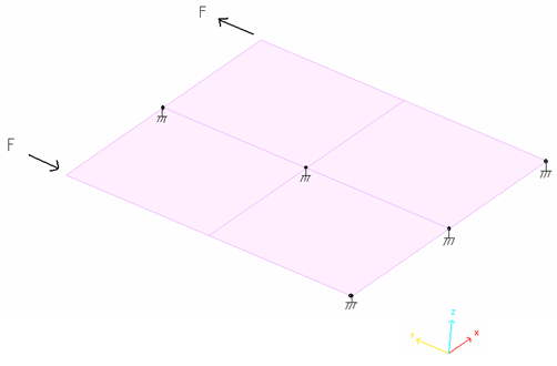
Figure 1. Boundary Conditions and Loads
Input Files
- 4Q4
- <install_directory>/hwsolvers/demos/radioss/example/18_Square_plate/Membrane_elasto-plastic/4Q4/.../TRACTION*
- 8T3
- <install_directory>/hwsolvers/demos/radioss/example/18_Square_plate/Membrane_elasto-plastic/8T3/.../TRACTION*
- 8T3 inv
- <install_directory>/hwsolvers/demos/radioss/example/18_Square_plate/Membrane_elasto-plastic/8T3_inv/.../TRACTION*
- 2Q4-4T3
- <install_directory>/hwsolvers/demos/radioss/example/18_Square_plate/Membrane_elasto-plastic/2Q4-4T3/.../TRACTION*
Model Description
Units: mm, ms, g, N, MPa
- Material Properties
- Initial density
- 7.8x10⁻³
- Young's modulus
- 210000
- Poisson ratio
- 0.3
- Yield stress
- 206
- Hardening parameter
- 450
- Hardening exponent
- 0.5
- Maximum stress
- 340
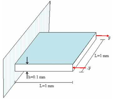
Figure 2. Geometry of the Problem
Model Method
- Mesh 1
- Two quadrilateral shells and four triangular shells (2Q4-4T3)
- Mesh 2
- Four quadrilateral shells (4Q4)
- Mesh 3
- Eight triangular shells (8T3)
- Mesh 4
- Eight triangular shells (8T3 inverse)
- QBAT formulation (Ishell =12)
- QEPH formulation (Ishell =24)
- Belytshcko & Tsay formulation (Ishell =1 or 3, hourglass control TYPE1, TYPE3)
- C0 and DKT18 formulations
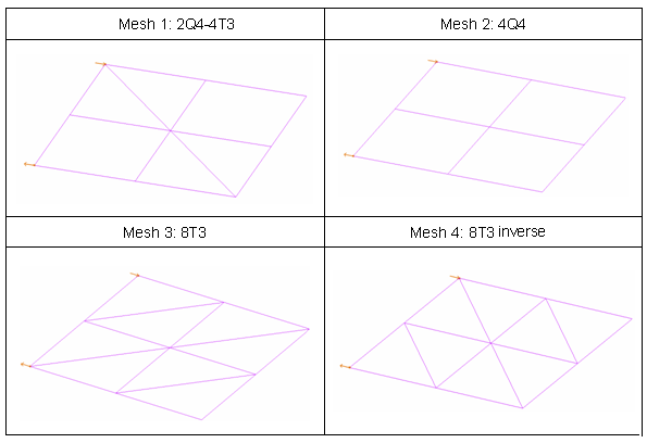
Figure 3. Square Plate Meshes
Results
Curves and Animations
- the use of different element formulations for each mesh
- the different types of mesh for a given element formulation
- absorbed energy (internal and hourglass)
- vertical displacement of the node under the loading point
The following diagrams summarize the results obtained.
Energy Curves / Comparison for Element Formulations
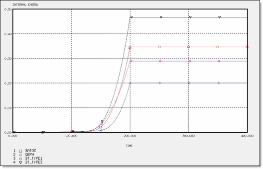
Figure 4. Internal Energy for 2 x Q4 and 4 x T3 Elements
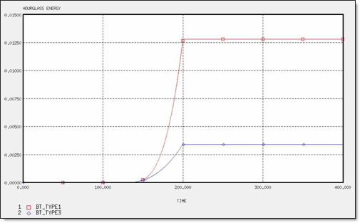
Figure 5. Hourglass Energy for 2 x Q4 and 4 x T3 Elements
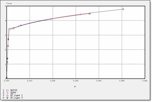
Figure 6. Force for 4 x Q4 Elements
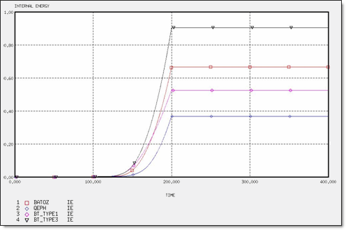
Figure 7. Internal Energy for 4 x Q4 Elements

Figure 8. Hourglass Energy for 4 x Q4 Elements
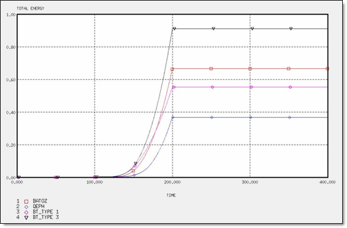
Figure 9. Total Energy for 4 x Q4 Elements
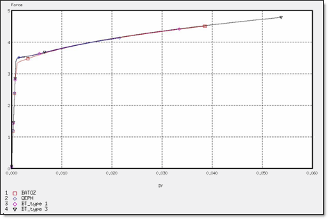
Figure 10. Force for 4 x Q4 Elements
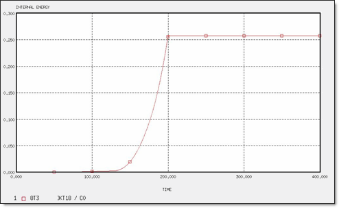
Figure 11. Internal Energy for 8 x T3 Elements
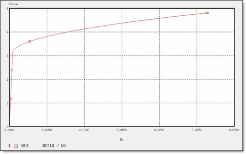
Figure 12. Force for 8 x T3 Elements
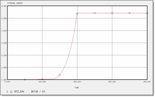
Figure 13. Internal Energy for 8 x T3 Elements (inversed mesh)
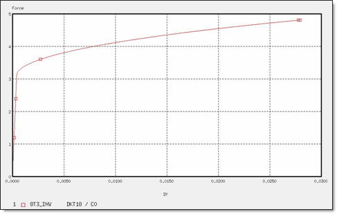
Figure 14. Force for 8 x T3 Elements (inversed mesh)
Comparison for Different Meshes
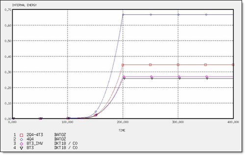
Figure 15. Internal Energy for Different Meshes
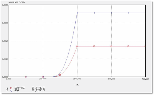
Figure 16. Hourglass Energy for Different Meshes
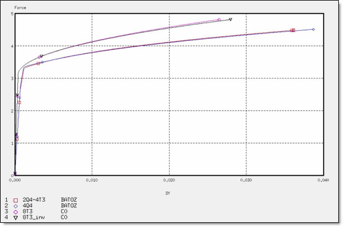
Figure 17. Force for Different Meshes
| Plastic | 2Q4-4T3 | 4Q4 | 8T3 | 8T3_INV | ||||||||
|---|---|---|---|---|---|---|---|---|---|---|---|---|
| QEPH | BT_TYPE 1 | BT_TYPE 3 | BATOZ | QEPH | BT_TYPE 1 | BT_TYPE 3 | BATOZ | DKT | CO | DKT | CO | |
| IEmax | 2.37 x 10⁻¹ | 2.89 x 10⁻¹ | 3.03 x 10⁻¹ | 3.46 x 10⁻¹ | 2.69 x 10⁻¹ | 5.27 x 10⁻¹ | 5.67 x 10⁻¹ | 6.67 x 10⁻¹ | 2.57 x 10⁻¹ | 2.57 x 10⁻¹ | 2.70 x 10⁻¹ | 2.70 x 10⁻¹ |
| HEmax | -- | 1.26 x 10⁻² | 2.13 x 10⁻² | -- | -- | 2.66 x 10⁻² | 4.41 x 10⁻² | -- | -- | -- | -- | -- |
| Total Energy | 2.37 x 10⁻¹ | 3.02 x 10⁻¹ | 3.24 x 10⁻¹ | 3.46 x 10⁻¹ | 2.96 x 10⁻¹ | 5.54 x 10⁻¹ | 6.11 x 10⁻¹ | 6.67 x 10⁻¹ | 2.57 x 10⁻¹ | 2.57 x 10⁻¹ | 2.70 x 10⁻¹ | 2.70 x 10⁻¹ |
| Dymax | 2.36 x 10⁻² | 3.20 x 10⁻² | 3.35 x 10⁻² | 3.61 x 10⁻² | 1.72 x 10⁻² | 3.34 x 10⁻² | 3.56 x 10⁻² | 3.87 x 10⁻² | 2.64 x 10⁻² | 2.64 x 10⁻² | 2.79 x 10⁻² | 2.79 x 10⁻² |
| max | 2.76 x 10⁻² | 3.78 x 10⁻² | 3.97 x 10⁻² | 4.43 x 10⁻² | 1.87 x 10⁻² | 3.72 x 10⁻² | 3.97 x 10⁻² | 4.50 x 10⁻² | 6.28 x 10⁻² | 6.28 x 10⁻² | 6.28 x 10⁻² | 6.28 x 10⁻² |
Conclusion
The purpose of this example was to highlight the role of the elasto-plastic treatment when formulating Radioss shells. The in-plane plasticity was considered here. Regarding the applied boundary conditions and the Poisson effect on the plate, the test may be very severe with respect to the behavior of plastic in under-integrated elements.
In the case of a mesh with four quadrilaterals, the QBAT element always provides the best results as it allows four integration points to be put over the element. The plasticity computation over the integration points is thus more accurate. The under-integrated elements, having just one integration point at the center, allows only two integration points to be put through the width of the mesh. Another point concerns the role of Poisson's ratio in the plasticity computation. In fact, the QEPH element uses an analytical expression of the hourglass energy which takes into account the accurate expression in terms of the Poisson ratio (refer to the Radioss Theory Manual for further information). However, some approximations are induced in its elasto-plastic formulation, possibly influencing the results, especially for low levels of work-hardening. In the BT element formulation with a TYPE3 hourglass control, the Poisson ratio effect on the plastic part of the hourglass deformation is computed by a simplified expression which minimizes its role. In fact, the results obtained using BT_TYPE3 are slightly affected by the change in (use =0 for the example studied and compare the results obtained). The BT elements are generally more flexible and provide better results for a very coarse mesh.
For triangular meshes, the in-plane behavior of DKT18 should be noted as being the same as the T3C0 element. In fact, the elements are essentially different with respect to their bending behaviors.