RD-E: 1102 Strain Rate Effect

The strain rate effect is considered, and the influence of strain rate filtering studied.

The changes in the mechanical properties at different loading speeds are caused by the increasing speed of the flow stress. As the flow stress increases, the fracture elongation can increase or decrease depending on the material. This also changes the energy a component can absorb in the event of a fast load before failure. In this example, the material strain rate influence with and without filtering will be studied.

Options and Keywords Used

Input Files

The input files used in this example include:

<install_directory>/hwsolvers/demos/radioss/example/11_Tensile_Test/

Model Description

In RD-E: 1101 Elasto-plastic Material Law Characterization, modeling a material’s elasto-plastic behavior based on one material test was looked at. For dynamic problems, the stiffness of a material can depend on the rate of deformation or strain rate. In this example, how to model the stiffness of the material as a function of the strain rate is outlined. First /MAT/LAW2 will be used with two coefficients that scale the stress strain curve depending on the strain rate. Next, test data at different strain rates is used with /MAT/LAW36 to model strain rate behavior of the material. The equivalent strain rate of each element is available as a contour output using the /ANIM/ELEM/EPSD or /H3D/ELEM/EPSD output request.

The strain rate of a tensile test is calculated by dividing the velocity of the gauge region by the gauge length. In this model, the gauge length is measured from node 102 to node 616 and is 80 mm. The displacement and velocity of node 616 is output relative to a moving coordinate (/FRAME/MOV) attached to node 102. Thus, the displacement and velocity of the gauge length can be plotted directly from the relative displacement and velocity of node 616.

Units: mm, ms, kg, N, GPa

Since the time unit is ms, the strain rate unit used in the model is: 1 ms  or ms 1 MathType@MTEF@5@5@+= feaagKart1ev2aqatCvAUfeBSjuyZL2yd9gzLbvyNv2CaerbuLwBLn hiov2DGi1BTfMBaeXatLxBI9gBaerbd9wDYLwzYbItLDharqqtubsr 4rNCHbGeaGqiVu0Je9sqqrpepC0xbbL8F4rqqrFfpeea0xe9Lq=Jc9 vqaqpepm0xbba9pwe9Q8fs0=yqaqpepae9pg0FirpepeKkFr0xfr=x fr=xb9adbaqaaeGaciGaaiaabeqaamaabaabaaGcbaWaaSaaaeaaca aIXaaabaGaamyBaiaadohaaaGaaeiiaiaab+gacaqGYbGaaeiiaiaa b2gacaqGZbWaaWbaaSqabeaacqGHsislcaaIXaaaaaaa@3F94@

/MAT/LAW2

The Johnson-Cook plasticity model (/MAT/LAW2) is used to consider the strain rate effect on the elasto-plastic.

The law reads as:(1) σ tr = ( a+b ε p n ) ( 1+c ln ε ˙ ε ˙ 0 ) MathType@MTEF@5@5@+= feaagKart1ev2aqatCvAUfeBSjuyZL2yd9gzLbvyNv2CaerbuLwBLn hiov2DGi1BTfMBaeXatLxBI9gBaerbd9wDYLwzYbItLDharqqtubsr 4rNCHbGeaGqiVCI8FfYJH8YrFfeuY=Hhbbf9v8qqaqFr0xc9pk0xbb a9q8WqFfeaY=biLkVcLq=JHqpepeea0=as0Fb9pgeaYRXxe9vr0=vr 0=vqpWqaaeaabiGaciaacaqabeaadaqaaqaaaOqaaabaaaaaaaaape Gaeq4Wdm3aaSbaaSqaaiaadshacaWGYbaabeaakiabg2da9iaaccka daqadaWdaeaapeGaamyyaiabgUcaRiaadkgacqGHflY1cqaH1oqzpa Waa0baaSqaa8qacaWGWbaapaqaa8qacaWGUbaaaaGccaGLOaGaayzk aaGaaiiOamaabmaapaqaa8qacaaIXaGaey4kaSIaam4yaiaacckaca WGSbGaamOBamaalaaapaqaa8qacuaH1oqzpaGbaiaaaeaacuaH1oqz gaGaamaaBaaaleaacaaIWaaabeaaaaaak8qacaGLOaGaayzkaaaaaa@53BB@
Where,
ε ˙
Strain rate
ε ˙ 0
Reference strain rate
c MathType@MTEF@5@5@+= feaagKart1ev2aaatCvAUfeBSjuyZL2yd9gzLbvyNv2CaerbwvMCKf MBHbqefqvATv2CG4uz3bIuV1wyUbqedmvETj2BSbqefm0B1jxALjhi ov2DaebbnrfifHhDYfgasaacH8srps0lbbf9q8WrFfeuY=Hhbbf9v8 qqaqFr0xc9pk0xbba9q8WqFfea0=yr0RYxir=Jbba9q8aq0=yq=He9 q8qqQ8frFve9Fve9Ff0dmeaacaGacmGadaWaaiqacaabaiaafaaake aacaWGJbaaaa@39BF@
Strain rate coefficient

The ( 1+c ln ε ˙ ε ˙ 0 ) MathType@MTEF@5@5@+= feaagKart1ev2aqatCvAUfeBSjuyZL2yd9gzLbvyNv2CaerbuLwBLn hiov2DGi1BTfMBaeXatLxBI9gBaerbd9wDYLwzYbItLDharqqtubsr 4rNCHbGeaGqiVCI8FfYJH8YrFfeuY=Hhbbf9v8qqaqFr0xc9pk0xbb a9q8WqFfeaY=biLkVcLq=JHqpepeea0=as0Fb9pgeaYRXxe9vr0=vr 0=vqpWqaaeaabiGaciaacaqabeaadaqaaqaaaOqaaabaaaaaaaaape WaaeWaa8aabaWdbiaaigdacqGHRaWkcaWGJbGaaiiOaiaadYgacaWG UbWaaSaaa8aabaWdbiqbew7aL9aagaGaaaqaaiqbew7aLzaacaWaaS baaSqaaiaaicdaaeqaaaaaaOWdbiaawIcacaGLPaaaaaa@41DF@ term scales the stress strain curve for strain rates that are greater than the reference strain rate.

For strain rates less than the reference strain rate, there is no scaling. In this example, there is no test data, so approximate values of ε ˙ 0 = 1x10⁻⁴ ms-1 and c MathType@MTEF@5@5@+= feaagKart1ev2aaatCvAUfeBSjuyZL2yd9gzLbvyNv2CaerbwvMCKf MBHbqefqvATv2CG4uz3bIuV1wyUbqedmvETj2BSbqefm0B1jxALjhi ov2DaebbnrfifHhDYfgasaacH8srps0lbbf9q8WrFfeuY=Hhbbf9v8 qqaqFr0xc9pk0xbba9q8WqFfea0=yr0RYxir=Jbba9q8aq0=yq=He9 q8qqQ8frFve9Fve9Ff0dmeaacaGacmGadaWaaiqacaabaiaafaaake aacaWGJbaaaa@39BF@ = 0.05 are used to demonstrate the behavior. When the strain rate behavior of the material is not known, the strain rate coefficient is typically defined as c MathType@MTEF@5@5@+= feaagKart1ev2aaatCvAUfeBSjuyZL2yd9gzLbvyNv2CaerbwvMCKf MBHbqefqvATv2CG4uz3bIuV1wyUbqedmvETj2BSbqefm0B1jxALjhi ov2DaebbnrfifHhDYfgasaacH8srps0lbbf9q8WrFfeuY=Hhbbf9v8 qqaqFr0xc9pk0xbba9q8WqFfea0=yr0RYxir=Jbba9q8aq0=yq=He9 q8qqQ8frFve9Fve9Ff0dmeaacaGacmGadaWaaiqacaabaiaafaaake aacaWGJbaaaa@39BF@ =0 and; thus, there is no strain rate effect for the material.

For further explanations about the Johnson-Cook model, refer to Elastic-plasticity of Isotropic Materials in the Radioss Theory Manual.


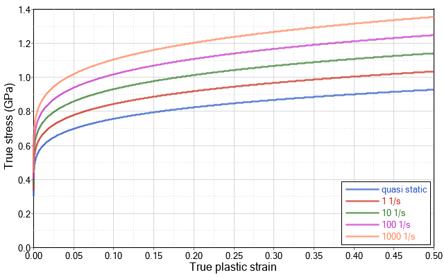
Figure 1. True Stress versus True Plastic Strain at Different Strain Rates for the Johnson-Cook Material Model

/MAT/LAW36

The second model uses the isotropic elasto-plastic material /MAT/LAW36 (PLAS_TAB) where user-defined stress versus plastic strain functions for different strain rates are derived from the real tests. 2 LAW36 will then use a linear interpolation between two different strain rate functions to calculate the material response for a particular strain rate. The input data for the material card is based on strain rate dependent test curves Figure 2.


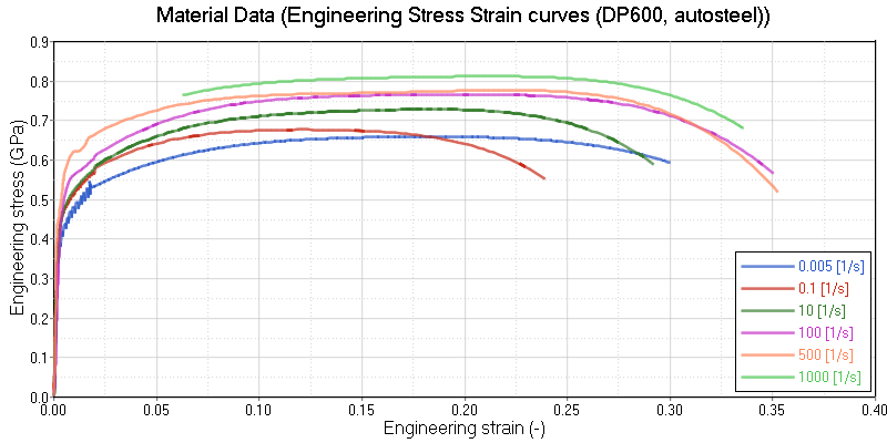
Figure 2. Material Data of Engineering Stress versus Strain for Different Strain Rates. (Steel DP600, original data from autosteel)
Due to high oscillation and other effects in the tested material (Figure 2), the curves must be modified in order to maintain numerical stability. In this example, the quasi-static curve was chosen as the initial curve and was shifted upwards until the best visual correlation to the other tested strain rate dependent curves was reached. This method avoids the intersections of different curves at higher strain rate regions (Figure 3 and Figure 4). The stress strain for each strain rate must not intersect.


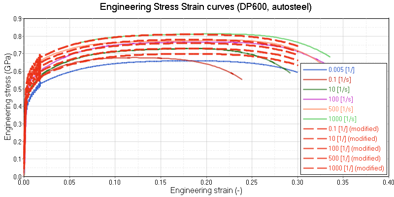
Figure 3. Original and Modified Engineering Stress versus Strain Curves for Different Strain Rates. (Steel DP600, autosteel)


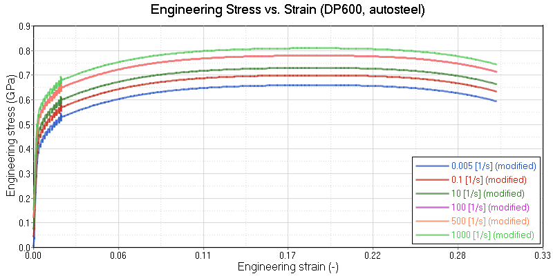
Figure 4. Modified Engineering Stress Strain Curves for Different Strain Rates
The true stress strain curves were derived from these new modified engineering stress strain curves. These curves were cut at the maximum stress and extrapolated to 100%. The same process described in RD-E: 1101 Elasto-plastic Material Law Characterization for LAW36 was used for each curve to create the following true stress versus plastic strain curves for use in /MAT/LAW36.


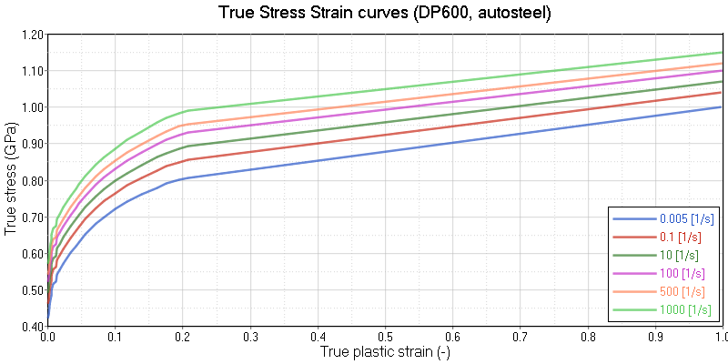
Figure 5. True Stress versus True Plastic Strain Curves for Different Strain Rates

Results

Because of the numerical application of the dynamic loadings, the strain rates are highly oscillating. This can lead to noisy results in the actual and local stress response. To obtain smooth and more physical stress results activate strain rate filtering by setting Fsmooth = 1 and defining a cutoff frequency using Fcut.

The strain rate is filtered using an exponential moving average filter.(2) ε ˙ f ( t )=a ε ˙ ( t )+( 1a ) ε ˙ ( tdt ) MathType@MTEF@5@5@+= feaagKart1ev2aaatCvAUfeBSjuyZL2yd9gzLbvyNv2CaerbuLwBLn hiov2DGi1BTfMBaeXatLxBI9gBaerbd9wDYLwzYbItLDharqqtubsr 4rNCHbGeaGqiVu0Je9sqqrpepC0xbbL8F4rqqrFfpeea0xe9Lq=Jc9 vqaqpepm0xbba9pwe9Q8fs0=yqaqpepae9pg0FirpepeKkFr0xfr=x fr=xb9adbaqaaeGaciGaaiaabeqaamaabaabaaGcbaaeaaaaaaaaa8 qacuaH1oqzpaGbaiaadaWgaaWcbaWdbiaadAgaa8aabeaak8qadaqa daWdaeaapeGaamiDaaGaayjkaiaawMcaaiabg2da9iaadggacuaH1o qzpaGbaiaapeWaaeWaa8aabaWdbiaadshaaiaawIcacaGLPaaacqGH RaWkdaqadaWdaeaapeGaaGymaiabgkHiTiaadggaaiaawIcacaGLPa aacuaH1oqzpaGbaiaapeWaaeWaa8aabaWdbiaadshacqGHsislcaWG KbGaamiDaaGaayjkaiaawMcaaaaa@4E79@
Where,
a=2π dt  F cut MathType@MTEF@5@5@+= feaagKart1ev2aaatCvAUfeBSjuyZL2yd9gzLbvyNv2CaerbuLwBLn hiov2DGi1BTfMBaeXatLxBI9gBaerbd9wDYLwzYbItLDharqqtubsr 4rNCHbGeaGqiVu0Je9sqqrpepC0xbbL8F4rqqrFfpeea0xe9Lq=Jc9 vqaqpepm0xbba9pwe9Q8fs0=yqaqpepae9pg0FirpepeKkFr0xfr=x fr=xb9adbaqaaeGaciGaaiaabeqaamaabaabaaGcbaaeaaaaaaaaa8 qacaWGHbGaeyypa0JaaGOmaiabec8aWjaacckacaWGKbGaamiDaiaa cckacaWGgbWdamaaBaaaleaapeGaam4yaiaadwhacaWG0baapaqaba aaaa@42A5@
dt MathType@MTEF@5@5@+= feaagKart1ev2aaatCvAUfeBSjuyZL2yd9gzLbvyNv2CaerbuLwBLn hiov2DGi1BTfMBaeXatLxBI9gBaerbd9wDYLwzYbItLDharqqtubsr 4rNCHbGeaGqiVu0Je9sqqrpepC0xbbL8F4rqqrFfpeea0xe9Lq=Jc9 vqaqpepm0xbba9pwe9Q8fs0=yqaqpepae9pg0FirpepeKkFr0xfr=x fr=xb9adbaqaaeGaciGaaiaabeqaamaabaabaaGcbaaeaaaaaaaaa8 qacaWGKbGaamiDaaaa@37F8@
Timestep of the simulation
F cut MathType@MTEF@5@5@+= feaagKart1ev2aaatCvAUfeBSjuyZL2yd9gzLbvyNv2CaerbuLwBLn hiov2DGi1BTfMBaeXatLxBI9gBaerbd9wDYLwzYbItLDharqqtubsr 4rNCHbGeaGqiVu0Je9sqqrpepC0xbbL8F4rqqrFfpeea0xe9Lq=Jc9 vqaqpepm0xbba9pwe9Q8fs0=yqaqpepae9pg0FirpepeKkFr0xfr=x fr=xb9adbaqaaeGaciGaaiaabeqaamaabaabaaGcbaaeaaaaaaaaa8 qacaWGgbWdamaaBaaaleaapeGaam4yaiaadwhacaWG0baapaqabaaa aa@3A16@
Cutoff frequency
ε ˙ f MathType@MTEF@5@5@+= feaagKart1ev2aaatCvAUfeBSjuyZL2yd9gzLbvyNv2CaerbuLwBLn hiov2DGi1BTfMBaeXatLxBI9gBaerbd9wDYLwzYbItLDharqqtubsr 4rNCHbGeaGqiVu0Je9sqqrpepC0xbbL8F4rqqrFfpeea0xe9Lq=Jc9 vqaqpepm0xbba9pwe9Q8fs0=yqaqpepae9pg0FirpepeKkFr0xfr=x fr=xb9adbaqaaeGaciGaaiaabeqaamaabaabaaGcbaaeaaaaaaaaa8 qacuaH1oqzpaGbaiaadaWgaaWcbaWdbiaadAgaa8aabeaaaaa@390B@
Filtered strain rate

Thus, F cut = a 2π dt   MathType@MTEF@5@5@+= feaagKart1ev2aaatCvAUfeBSjuyZL2yd9gzLbvyNv2CaerbuLwBLn hiov2DGi1BTfMBaeXatLxBI9gBaerbd9wDYLwzYbItLDharqqtubsr 4rNCHbGeaGqiVu0Je9sqqrpepC0xbbL8F4rqqrFfpeea0xe9Lq=Jc9 vqaqpepm0xbba9pwe9Q8fs0=yqaqpepae9pg0FirpepeKkFr0xfr=x fr=xb9adbaqaaeGaciGaaiaabeqaamaabaabaaGcbaaeaaaaaaaaa8 qacaWGgbWdamaaBaaaleaapeGaam4yaiaadwhacaWG0baapaqabaGc peGaeyypa0ZaaSaaaeaacaWGHbaabaGaaGOmaiabec8aWjaacckaca WGKbGaamiDaaaacaGGGcaaaa@42CF@

The cutoff frequency is a function of the model timestep. Experience shows that the speed of the deformation is important also. For slower speeds like a car crash, 1 – 10 kHz (1000 – 10,000 Hz) is a good value, but for high-speed events, like ballistic, less filtering should be used, so 1 – 10 GHz is appropriate. Good engineering judgment should be used to determine a good value for each simulation.

/MAT/LAW2 with Strain Rate Effect

Starting with the LAW2 material input from RD-E: 1101 Elasto-plastic Material Law Characterization, strain rate input was defined ε ˙ 0 = 1x10⁻⁴ ms-1 and c MathType@MTEF@5@5@+= feaagKart1ev2aaatCvAUfeBSjuyZL2yd9gzLbvyNv2CaerbwvMCKf MBHbqefqvATv2CG4uz3bIuV1wyUbqedmvETj2BSbqefm0B1jxALjhi ov2DaebbnrfifHhDYfgasaacH8srps0lbbf9q8WrFfeuY=Hhbbf9v8 qqaqFr0xc9pk0xbba9q8WqFfea0=yr0RYxir=Jbba9q8aq0=yq=He9 q8qqQ8frFve9Fve9Ff0dmeaacaGacmGadaWaaiqacaabaiaafaaake aacaWGJbaaaa@39BF@ = 0.05 to demonstrate the functionality (Figure 6 and Figure 7).


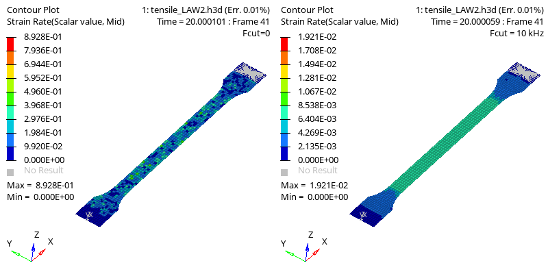
Figure 6. Comparison of the Distribution of the Strain Rate in the Specimen without Strain Rate Filtering (Fcut=0) . and with strain rate filtering (Fsmooth=1 and Fcut=10 kHz)

The explicit scheme is an element-by-element method and the local treatment of temporal oscillations puts spatial oscillations into the model. A more physical strain rate distribution is achieved by filtering. Moreover, such results show oscillations in the stress strain curve when not damped by filtering.

The strain rate of the entire tensile test can be calculated by dividing the velocity of the gauge length (velocity of node 616) by the gauge length (80 mm) which results in a strain rate, which ranges from 0.0075 ms-1 at the start of the simulation to 0.01 ms-1 at the end of the simulation. This corresponds well with the strain rate contour plot with strain rate filtering. Since the simulation strain rate speed is larger than the reference strain rate, ε ˙ 0 = 1x10⁻⁴ ms-1 the material response is stiffer (Figure 7).


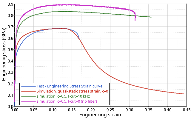
Figure 7. Engineering Stress Strain Curves with and without Strain Rate Filtering /MAT/LAW2

/MAT/LAW36 with Strain Rate Effect

Similar to /MAT/LAW2, the results are smoothed when the strain rate filter is used (Figure 8).


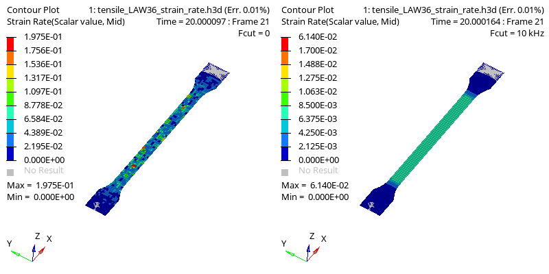
Figure 8. Comparison of the Distribution of the Strain Rate in the Specimen, with and without Strain Rate Filtering /MAT/LAW36
Similar to LAW2, the strain rate contour plot is similar to the strain rate calculated from the gauge length of the tensile test.


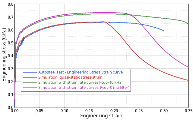
Figure 9. Comparison of the Distribution of the Strain Rate in the Specimen, with and without Strain Rate Filtering (/MAT/LAW36) . and engineering stress strain curves without strain rate

As shown in Figure 9, a strain rate larger than the quasi-static test causes the material to be stiffer. The quasi-static and case without a filter, experience material necking which results in the reduction in stress.

Conclusion

Strain rate effects are important in dynamic events. LAW2 includes 2 parameters that can be used to add strain rate effects to the model. LAW36 allows separate stress versus plastic strain functions to be defined for different strain rates. No matter which material model is used, it is important to use strain rate filtering to reduce numerical noise and smooth the response.