RD-E: 1101 Elasto-plastic Material Law Characterization

The purpose of this example is to introduce a method for characterizing and validation of the most commonly used Radioss material laws for modeling elasto-plastic materials.

The use of "engineering” and "true” stress-strain curves is pointed out. Failure models are also introduced to better fit the experimental response.

Options and Keywords Used

Input Files

The input files used in this example include:

<install_directory>/hwsolvers/demos/radioss/example/11_Tensile_test/

Model Description

Tension is applied to an object. The standardized “dogbone" object contains a defined cross-sectional area A 0 MathType@MTEF@5@5@+= feaagKart1ev2aaatCvAUfeBSjuyZL2yd9gzLbvyNv2CaerbuLwBLn hiov2DGi1BTfMBaeXatLxBI9gBaerbd9wDYLwzYbItLDharqqtubsr 4rNCHbGeaGqiVu0Je9sqqrpepC0xbbL8F4rqqrFfpeea0xe9Lq=Jc9 vqaqpepm0xbba9pwe9Q8fs0=yqaqpepae9pg0FirpepeKkFr0xfr=x fr=xb9adbaqaaeGaciGaaiaabeqaamaabaabaaGcbaGaamyqamaaBa aaleaacaaIWaaabeaaaaa@37A2@ . The material to be characterized is DP600 Steel. 1 A velocity is imposed at the right-end.

Units: mm, ms, kg, N, GPa.

rad_ex_fig_11-1
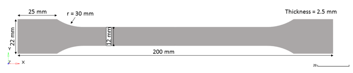
Figure 1. Geometry of the Standardized Tensile Object. with a defined cross-sectional area

The material undergoes isotropic elasto-plastic behavior which can be reproduced by a Johnson-Cook (/MAT/LAW2). The tabulated material law (/MAT/LAW36) is also studied.

The model is meshed with 4-node shells and 3-node shells as shown in Figure 2. The average element size is about 2 mm.

The shell properties use recommended best practice settings, except for the thickness which matches the test.
  • 5 integration points over the thickness.
  • QEPH shell formulation (Ishell = 24).
  • Iterative plasticity for plane stress (Newton-Raphson method; Iplas = 1).
  • Thickness changes are considered in stress computation (Ithick = 1).
  • Initial thickness is uniform, equal to 2.5 mm

Boundary Condition

The left side of the object is fixed in all six degrees of freedom (all three translational and all three rotational DOFs). On the right side only translation in X-direction is free, all other five DOFs are fixed. An imposed velocity of -1.0 m/s in the X-direction is applied to the main node of the rigid body, shown Figure 2, whereby the elongation is increased uniformly at low speed.


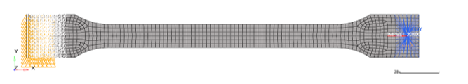
Figure 2. All Boundary Conditions Applied to the Tensile Test Model

Two measurement nodes with a distance of 80 mm are chosen (Figure 3) to continuously measure the change in length Δ l MathType@MTEF@5@5@+= feaagKart1ev2aaatCvAUfeBSjuyZL2yd9gzLbvyNv2CaerbwvMCKf MBHbqefqvATv2CG4uz3bIuV1wyUbqedmvETj2BSbqefm0B1jxALjhi ov2DaebbnrfifHhDYfgasaacH8srps0lbbf9q8WrFfeuY=Hhbbf9v8 qqaqFr0xc9pk0xbba9q8WqFfea0=yr0RYxir=Jbba9q8aq0=yq=He9 q8qqQ8frFve9Fve9Ff0dmeaacaGacmGadaWaaiqacaabaiaafaaake aacqqHuoarcaWGSbaaaa@3B2E@ in the measurement section of the sample during the simulation and to obtain the strain ε e MathType@MTEF@5@5@+= feaagKart1ev2aqatCvAUfeBSjuyZL2yd9gzLbvyNv2CaerbuLwBLn hiov2DGi1BTfMBaeXatLxBI9gBaerbd9wDYLwzYbItLDharqqtubsr 4rNCHbGeaGqiVu0Je9sqqrpepC0xbbL8F4rqqrFfpeea0xe9Lq=Jc9 vqaqpepm0xbbG8FasPYRqj0=yi0dXdbba9pGe9xq=JbbG8A8frFve9 Fve9Ff0dmeaabaqaciGacaGaaeqabaWaaeaaeaaakeaaqaaaaaaaaa Wdbiabew7aL9aadaWgaaWcbaWdbiaadwgaa8aabeaaaaa@396A@ on the sample.

The engineering (nominal) stress is calculated as:(1) σ e =   F A 0 MathType@MTEF@5@5@+= feaagKart1ev2aqatCvAUfeBSjuyZL2yd9gzLbvyNv2CaerbuLwBLn hiov2DGi1BTfMBaeXatLxBI9gBaerbd9wDYLwzYbItLDharqqtubsr 4rNCHbGeaGqiVu0Je9sqqrpepC0xbbL8F4rqqrFfpeea0xe9Lq=Jc9 vqaqpepm0xbbG8FasPYRqj0=yi0dXdbba9pGe9xq=JbbG8A8frFve9 Fve9Ff0dmeaabaqaciGacaGaaeqabaWaaeaaeaaakeaaqaaaaaaaaa Wdbiabeo8aZ9aadaWgaaWcbaWdbiaadwgaa8aabeaak8qacqGH9aqp caGGGcWaaSaaaeaacaWGgbaabaGaamyqa8aadaWgaaWcbaWdbiaaic daa8aabeaaaaaaaa@3E7F@ Where,
F MathType@MTEF@5@5@+= feaagKart1ev2aqatCvAUfeBSjuyZL2yd9gzLbvyNv2CaerbuLwBLn hiov2DGi1BTfMBaeXatLxBI9gBaerbd9wDYLwzYbItLDharqqtubsr 4rNCHbGeaGqiVu0Je9sqqrpepC0xbbL8F4rqqrFfpeea0xe9Lq=Jc9 vqaqpepm0xbbG8FasPYRqj0=yi0dXdbba9pGe9xq=JbbG8A8frFve9 Fve9Ff0dmeaabaqaciGacaGaaeqabaWaaeaaeaaakabaaaaaaaaape qaaiaadAeaaaa@374A@
Measure force
A 0 MathType@MTEF@5@5@+= feaagKart1ev2aqatCvAUfeBSjuyZL2yd9gzLbvyNv2CaerbuLwBLn hiov2DGi1BTfMBaeXatLxBI9gBaerbd9wDYLwzYbItLDharqqtubsr 4rNCHbGeaGqiVu0Je9sqqrpepC0xbbL8F4rqqrFfpeea0xe9Lq=Jc9 vqaqpepm0xbbG8FasPYRqj0=yi0dXdbba9pGe9xq=JbbG8A8frFve9 Fve9Ff0dmeaabaqaciGacaGaaeqabaWaaeaaeaaakabaaaaaaaaape qaaiaadgeapaWaaSbaaSqaa8qacaaIWaaapaqabaaaaa@3859@
Cross-sectional area of the undeformed sample
The total engineering strain is calculated as:(2) ε e =   Δ l l 0 MathType@MTEF@5@5@+= feaagKart1ev2aqatCvAUfeBSjuyZL2yd9gzLbvyNv2CaerbuLwBLn hiov2DGi1BTfMBaeXatLxBI9gBaerbd9wDYLwzYbItLDharqqtubsr 4rNCHbGeaGqiVCI8FfYJH8YrFfeuY=Hhbbf9v8qqaqFr0xc9pk0xbb a9q8WqFfeaY=biLkVcLq=JHqpepeea0=as0Fb9pgeaYRXxe9vr0=vr 0=vqpWqaaeaabiGaciaacaqabeaadaqaaqaaaOqaaabaaaaaaaaape GaeqyTdu2damaaBaaaleaapeGaamyzaaWdaeqaaOWdbiabg2da9iaa cckadaWcaaWdaeaapeGaeuiLdqKaamiBaaWdaeaapeGaamiBa8aada WgaaWcbaWdbiaaicdaa8aabeaaaaaaaa@3FE5@ Where,
Δ l MathType@MTEF@5@5@+= feaagKart1ev2aqatCvAUfeBSjuyZL2yd9gzLbvyNv2CaerbuLwBLn hiov2DGi1BTfMBaeXatLxBI9gBaerbd9wDYLwzYbItLDharqqtubsr 4rNCHbGeaGqiVCI8FfYJH8YrFfeuY=Hhbbf9v8qqaqFr0xc9pk0xbb a9q8WqFfeaY=biLkVcLq=JHqpepeea0=as0Fb9pgeaYRXxe9vr0=vr 0=vqpWqaaeaabiGaciaacaqabeaadaqaaqaaaOqaaabaaaaaaaaape GaeuiLdqKaamiBaaaa@3863@
Change in length between the two measurement points
l 0 MathType@MTEF@5@5@+= feaagKart1ev2aqatCvAUfeBSjuyZL2yd9gzLbvyNv2CaerbuLwBLn hiov2DGi1BTfMBaeXatLxBI9gBaerbd9wDYLwzYbItLDharqqtubsr 4rNCHbGeaGqiVCI8FfYJH8YrFfeuY=Hhbbf9v8qqaqFr0xc9pk0xbb a9q8WqFfeaY=biLkVcLq=JHqpepeea0=as0Fb9pgeaYRXxe9vr0=vr 0=vqpWqaaeaabiGaciaacaqabeaadaqaaqaaaOqaaabaaaaaaaaape GaamiBa8aadaWgaaWcbaWdbiaaicdaa8aabeaaaaa@3811@
Initial length of the measurement section


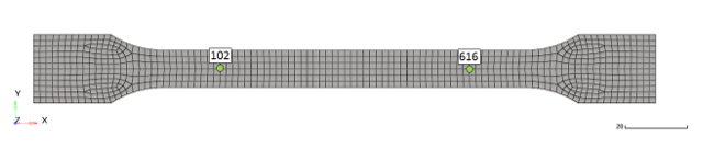
Figure 3. Measurement Nodes with a Distance of 80 mm
The true strain is computed with the relationship:(3) ε t r = 1 n ( 1 + Δ l / l 0 ) MathType@MTEF@5@5@+= feaagKart1ev2aaatCvAUfeBSjuyZL2yd9gzLbvyNv2CaerbwvMCKf MBHbqefqvATv2CG4uz3bIuV1wyUbqedmvETj2BSbqefm0B1jxALjhi ov2DaebbnrfifHhDYfgasaacH8srps0lbbf9q8WrFfeuY=Hhbbf9v8 qqaqFr0xc9pk0xbba9q8WqFfea0=yr0RYxir=Jbba9q8aq0=yq=He9 q8qqQ8frFve9Fve9Ff0dmeaacaGacmGadaWaaiqacaabaiaafaaake aacqaH1oqzdaWgaaWcbaGaamiDaiaadkhaaeqaaOGaeyypa0JaaGym aiGac6gadaqadaqaaiaaigdacqGHRaWkcaqGuoGaamiBaiaac+caca WGSbWaaSbaaSqaaiaaicdaaeqaaaGccaGLOaGaayzkaaaaaa@471E@
Engineering strain and true strain; therefore, are linked together by:(4) ε t r = 1 n ( 1 + ε e ) MathType@MTEF@5@5@+= feaagKart1ev2aaatCvAUfeBSjuyZL2yd9gzLbvyNv2CaerbwvMCKf MBHbqefqvATv2CG4uz3bIuV1wyUbqedmvETj2BSbqefm0B1jxALjhi ov2DaebbnrfifHhDYfgasaacH8srps0lbbf9q8WrFfeuY=Hhbbf9v8 qqaqFr0xc9pk0xbba9q8WqFfea0=yr0RYxir=Jbba9q8aq0=yq=He9 q8qqQ8frFve9Fve9Ff0dmeaacaGacmGadaWaaiqacaabaiaafaaake aacqaH1oqzdaWgaaWcbaGaamiDaiaadkhaaeqaaOGaeyypa0JaaGym aiGac6gadaqadaqaaiaaigdacqGHRaWkcqaH1oqzdaWgaaWcbaGaam yzaaqabaaakiaawIcacaGLPaaaaaa@4546@
True stresses are measured by dividing the force with the true deformed section:(5) σ tr =  F A MathType@MTEF@5@5@+= feaagKart1ev2aqatCvAUfeBSjuyZL2yd9gzLbvyNv2CaerbuLwBLn hiov2DGi1BTfMBaeXatLxBI9gBaerbd9wDYLwzYbItLDharqqtubsr 4rNCHbGeaGqiVCI8FfYJH8YrFfeuY=Hhbbf9v8qqaqFr0xc9pk0xbb a9q8WqFfeaY=biLkVcLq=JHqpepeea0=as0Fb9pgeaYRXxe9vr0=vr 0=vqpWqaaeaabiGaciaacaqabeaadaqaaqaaaOqaaabaaaaaaaaape Gaeq4Wdm3damaaBaaaleaapeGaamiDaiaadkhaa8aabeaak8qacqGH 9aqpcaGGGcWaaSaaa8aabaWdbiaadAeaa8aabaWdbiaadgeaaaaaaa@3E3C@
Thus, to compute true stresses, the area variation must be considered. If Poisson’s coefficient is 0.5 during plastic deformation, the true area in mono-axial traction is:(6) A =   A 0 × e x p ( ε t r ) MathType@MTEF@5@5@+= feaagKart1ev2aqatCvAUfeBSjuyZL2yd9gzLbvyNv2CaerbuLwBLn hiov2DGi1BTfMBaeXatLxBI9gBaerbd9wDYLwzYbItLDharqqtubsr 4rNCHbGeaGqiVCI8FfYJH8YrFfeuY=Hhbbf9v8qqaqFr0xc9pk0xbb a9q8WqFfeaY=biLkVcLq=JHqpepeea0=as0Fb9pgeaYRXxe9vr0=vr 0=vqpWqaaeaabiGaciaacaqabeaadaqaaqaaaOqaaabaaaaaaaaape Gaamyqaiabg2da9iaacckacaWGbbWdamaaBaaaleaapeGaaGimaaWd aeqaaOGaey41aq7dbiaadwgacaWG4bGaamiCamaabmaapaqaa8qacq GHsislcqaH1oqzpaWaaSbaaSqaa8qacaWG0bGaamOCaaWdaeqaaaGc peGaayjkaiaawMcaaaaa@4683@
Thus, the relationship between true and engineering stresses is:(7) σ t r =   σ e × e x p ( ε t r ) MathType@MTEF@5@5@+= feaagKart1ev2aqatCvAUfeBSjuyZL2yd9gzLbvyNv2CaerbuLwBLn hiov2DGi1BTfMBaeXatLxBI9gBaerbd9wDYLwzYbItLDharqqtubsr 4rNCHbGeaGqiVCI8FfYJH8YrFfeuY=Hhbbf9v8qqaqFr0xc9pk0xbb a9q8WqFfeaY=biLkVcLq=JHqpepeea0=as0Fb9pgeaYRXxe9vr0=vr 0=vqpWqaaeaabiGaciaacaqabeaadaqaaqaaaOqaaabaaaaaaaaape Gaeq4Wdm3damaaBaaaleaapeGaamiDaiaadkhaa8aabeaak8qacqGH 9aqpcaGGGcGaeq4Wdm3damaaBaaaleaapeGaamyzaaWdaeqaaOGaey 41aq7dbiaadwgacaWG4bGaamiCamaabmaapaqaa8qacqaH1oqzpaWa aSbaaSqaa8qacaWG0bGaamOCaaWdaeqaaaGcpeGaayjkaiaawMcaaa aa@4A24@


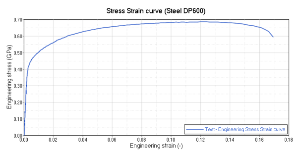
Figure 4. Experimental Results of a Tensile Test of a DP600 Steel Object

Characterization of the Material Law

There are two steps to characterize the material law.

Transform the engineering stress versus engineering strain curve into a true stress versus true strain curve (this step applies to any elasto-plastic material law).

Extract the main parameters from the true stress versus true strain curve, to define the material law (Johnson-Cook law and material coefficients for /MAT/LAW2 or the yield curve definition for /MAT/LAW36).

When there is no material test data available (e.g. in an early design stage), values of Yield stress, Ultimate tensile strength (engineering stress value) and Engineering strain at UTS must be provided to characterize /MAT/LAW2 using Iflag = 1.

The characterization will be made for /MAT/LAW2 (Johnson-Cook elasto-plastic), and /MAT/LAW36 (tabulated elasto-plastic). For each of the material laws, the yield stress and Young's modulus are determined from the curve.

The plastic strain can be defined as:(8) ε pl =  ε tr σ tr E   MathType@MTEF@5@5@+= feaagKart1ev2aqatCvAUfeBSjuyZL2yd9gzLbvyNv2CaerbuLwBLn hiov2DGi1BTfMBaeXatLxBI9gBaerbd9wDYLwzYbItLDharqqtubsr 4rNCHbGeaGqiVu0Je9sqqrpepC0xbbL8F4rqqrFfpeea0xe9Lq=Jc9 vqaqpepm0xbbG8FasPYRqj0=yi0dXdbba9pGe9xq=JbbG8A8frFve9 Fve9Ff0dmeaabaqaciGacaGaaeqabaWaaeaaeaaakeaaqaaaaaaaaa Wdbiabew7aL9aadaWgaaWcbaWdbiaadchacaWGSbaapaqabaGcpeGa eyypa0JaaiiOaiabew7aL9aadaWgaaWcbaWdbiaadshacaWGYbaapa qabaGcpeGaeyOeI0YaaSaaaeaacqaHdpWCpaWaaSbaaSqaa8qacaWG 0bGaamOCaaWdaeqaaaGcpeqaaiaadweaaaGaaiiOaaaa@47C7@
An important point to be characterized on the curve is the necking point, where the slope of the force versus the displacement curve is equal to 0, and where the following relationships apply:(9) σ t r ε t r σ t r F δ = 0 MathType@MTEF@5@5@+= feaagKart1ev2aaatCvAUfeBSjuyZL2yd9gzLbvyNv2CaerbwvMCKf MBHbqefqvATv2CG4uz3bIuV1wyUbqedmvETj2BSbqefm0B1jxALjhi ov2DaebbnrfifHhDYfgasaacH8srps0lbbf9q8WrFfeuY=Hhbbf9v8 qqaqFr0xc9pk0xbba9q8WqFfea0=yr0RYxir=Jbba9q8aq0=yq=He9 q8qqQ8frFve9Fve9Ff0dmeaacaGacmGadaWaaiqacaabaiaafaaake aadaWcaaqaaiabgkGi2kabeo8aZnaaBaaaleaacaWG0bGaamOCaaqa baaakeaacqGHciITcqaH1oqzdaahaaWcbeqaaiaadshacaWGYbaaaa aakiabgIKi7kabeo8aZnaaBaaaleaacaWG0bGaamOCaaqabaGccaaM f8+aaSaaaeaacqGHciITcaWGgbaabaGaeyOaIyRaeqiTdqgaaiabg2 da9iaaicdaaaa@519E@

rad_ex_fig_11-8
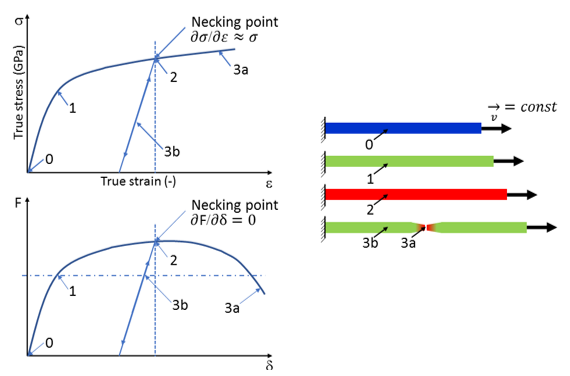
Figure 5. Tensile Test Schematic. (0 - 1= elastic region; 1= yield point; 2= necking point; 3a= fracture; 3b= linear elastic relaxation)
Table 1. Equations Used for Analysis
Material Property Generic Equation
Engineering stress σ e =  F A 0 MathType@MTEF@5@5@+= feaagKart1ev2aqatCvAUfeBSjuyZL2yd9gzLbvyNv2CaerbuLwBLn hiov2DGi1BTfMBaeXatLxBI9gBaerbd9wDYLwzYbItLDharqqtubsr 4rNCHbGeaGqiVCI8FfYJH8YrFfeuY=Hhbbf9v8qqaqFr0xc9pk0xbb a9q8WqFfeaY=biLkVcLq=JHqpepeea0=as0Fb9pgeaYRXxe9vr0=vr 0=vqpWqaaeaabiGaciaacaqabeaadaqaaqaaaOqaaabaaaaaaaaape Gaeq4Wdm3damaaBaaaleaapeGaamyzaaWdaeqaaOWdbiabg2da9iaa cckadaWcaaWdaeaapeGaamOraaWdaeaapeGaamyqa8aadaWgaaWcba Wdbiaaicdaa8aabeaaaaaaaa@3E4A@
Engineering strain ε e = Δ l l 0 MathType@MTEF@5@5@+= feaagKart1ev2aaatCvAUfeBSjuyZL2yd9gzLbvyNv2CaerbwvMCKf MBHbqefqvATv2CG4uz3bIuV1wyUbqedmvETj2BSbqefm0B1jxALjhi ov2DaebbnrfifHhDYfgasaacH8srps0lbbf9q8WrFfeuY=Hhbbf9v8 qqaqFr0xc9pk0xbba9q8WqFfea0=yr0RYxir=Jbba9q8aq0=yq=He9 q8qqQ8frFve9Fve9Ff0dmeaacaGacmGadaWaaiqacaabaiaafaaake aacqaH1oqzdaWgaaWcbaGaamyzaaqabaGccqGH9aqpdaWcaaqaaiaa bs5acaWGSbaabaGaamiBamaaBaaaleaacaaIWaaabeaaaaaaaa@4096@
True stress σ tr =  σ e exp( ε tr ) MathType@MTEF@5@5@+= feaagKart1ev2aqatCvAUfeBSjuyZL2yd9gzLbvyNv2CaerbuLwBLn hiov2DGi1BTfMBaeXatLxBI9gBaerbd9wDYLwzYbItLDharqqtubsr 4rNCHbGeaGqiVCI8FfYJH8YrFfeuY=Hhbbf9v8qqaqFr0xc9pk0xbb a9q8WqFfeaY=biLkVcLq=JHqpepeea0=as0Fb9pgeaYRXxe9vr0=vr 0=vqpWqaaeaabiGaciaacaqabeaadaqaaqaaaOqaaabaaaaaaaaape Gaeq4Wdm3damaaBaaaleaapeGaamiDaiaadkhaa8aabeaak8qacqGH 9aqpcaGGGcGaeq4Wdm3damaaBaaaleaapeGaamyzaaWdaeqaaOWdbi aadwgacaWG4bGaamiCamaabmaapaqaa8qacqaH1oqzpaWaaSbaaSqa a8qacaWG0bGaamOCaaWdaeqaaaGcpeGaayjkaiaawMcaaaaa@480D@
True strain ε t r = 1 n ( 1 + ε e ) MathType@MTEF@5@5@+= feaagKart1ev2aaatCvAUfeBSjuyZL2yd9gzLbvyNv2CaerbwvMCKf MBHbqefqvATv2CG4uz3bIuV1wyUbqedmvETj2BSbqefm0B1jxALjhi ov2DaebbnrfifHhDYfgasaacH8srps0lbbf9q8WrFfeuY=Hhbbf9v8 qqaqFr0xc9pk0xbba9q8WqFfea0=yr0RYxir=Jbba9q8aq0=yq=He9 q8qqQ8frFve9Fve9Ff0dmeaacaGacmGadaWaaiqacaabaiaafaaake aacqaH1oqzdaWgaaWcbaGaamiDaiaadkhaaeqaaOGaeyypa0JaaGym aiGac6gadaqadaqaaiaaigdacqGHRaWkcqaH1oqzdaWgaaWcbaGaam yzaaqabaaakiaawIcacaGLPaaaaaa@4546@
True strain rate ε ˙ p l = Δ ε p l Δ t MathType@MTEF@5@5@+= feaagKart1ev2aaatCvAUfeBSjuyZL2yd9gzLbvyNv2CaerbwvMCKf MBHbqefqvATv2CG4uz3bIuV1wyUbqedmvETj2BSbqefm0B1jxALjhi ov2DaebbnrfifHhDYfgasaacH8srps0lbbf9q8WrFfeuY=Hhbbf9v8 qqaqFr0xc9pk0xbba9q8WqFfea0=yr0RYxir=Jbba9q8aq0=yq=He9 q8qqQ8frFve9Fve9Ff0dmeaacaGacmGadaWaaiqacaabaiaafaaake aacuaH1oqzgaGaamaaBaaaleaacaWGWbGaamiBaaqabaGccqGH9aqp daWcaaqaaiaabs5acqaH1oqzdaWgaaWcbaGaamiCaiaadYgaaeqaaa GcbaGaaeiLdiaadshaaaaaaa@44A9@

Results

/MAT/LAW2: Elasto-plastic Material Law using the Johnson-Cook Model

The stress versus plastic strain law is:(10) σ t r =   a + b ε p l n MathType@MTEF@5@5@+= feaagKart1ev2aqatCvAUfeBSjuyZL2yd9gzLbvyNv2CaerbuLwBLn hiov2DGi1BTfMBaeXatLxBI9gBaerbd9wDYLwzYbItLDharqqtubsr 4rNCHbGeaGqiVu0Je9sqqrpepC0xbbL8F4rqqrFfpeea0xe9Lq=Jc9 vqaqpepm0xbbG8FasPYRqj0=yi0dXdbba9pGe9xq=JbbG8A8frFve9 Fve9Ff0dmeaabaqaciGacaGaaeqabaWaaeaaeaaakeaaqaaaaaaaaa Wdbiabeo8aZ9aadaWgaaWcbaWdbiaadshacaWGYbaapaqabaGcpeGa eyypa0JaaiiOaiaadggacqGHRaWkcaWGIbGaeyyXICTaeqyTdu2dam aaBaaaleaapeGaamiCaiaadYgaa8aabeaakmaaCaaaleqabaWdbiaa d6gaaaaaaa@46EA@ Where,
a MathType@MTEF@5@5@+= feaagKart1ev2aqatCvAUfeBSjuyZL2yd9gzLbvyNv2CaerbuLwBLn hiov2DGi1BTfMBaeXatLxBI9gBaerbd9wDYLwzYbItLDharqqtubsr 4rNCHbGeaGqiVu0Je9sqqrpepC0xbbL8F4rqqrFfpeea0xe9Lq=Jc9 vqaqpepm0xbbG8FasPYRqj0=yi0dXdbba9pGe9xq=JbbG8A8frFve9 Fve9Ff0dmeaabaqaciGacaGaaeqabaWaaeaaeaaakeaaqaaaaaaaaa Wdbiaadggaaaa@3765@
Yield stress and is read from the experimental curve
b MathType@MTEF@5@5@+= feaagKart1ev2aqatCvAUfeBSjuyZL2yd9gzLbvyNv2CaerbuLwBLn hiov2DGi1BTfMBaeXatLxBI9gBaerbd9wDYLwzYbItLDharqqtubsr 4rNCHbGeaGqiVu0Je9sqqrpepC0xbbL8F4rqqrFfpeea0xe9Lq=Jc9 vqaqpepm0xbbG8FasPYRqj0=yi0dXdbba9pGe9xq=JbbG8A8frFve9 Fve9Ff0dmeaabaqaciGacaGaaeqabaWaaeaaeaaakeaaqaaaaaaaaa Wdbiaadggaaaa@3765@ and n MathType@MTEF@5@5@+= feaagKart1ev2aqatCvAUfeBSjuyZL2yd9gzLbvyNv2CaerbuLwBLn hiov2DGi1BTfMBaeXatLxBI9gBaerbd9wDYLwzYbItLDharqqtubsr 4rNCHbGeaGqiVu0Je9sqqrpepC0xbbL8F4rqqrFfpeea0xe9Lq=Jc9 vqaqpepm0xbbG8FasPYRqj0=yi0dXdbba9pGe9xq=JbbG8A8frFve9 Fve9Ff0dmeaabaqaciGacaGaaeqabaWaaeaaeaaakeaaqaaaaaaaaa Wdbiaadggaaaa@3765@
Material paraemters

If the material parameters b MathType@MTEF@5@5@+= feaagKart1ev2aqatCvAUfeBSjuyZL2yd9gzLbvyNv2CaerbuLwBLn hiov2DGi1BTfMBaeXatLxBI9gBaerbd9wDYLwzYbItLDharqqtubsr 4rNCHbGeaGqiVu0Je9sqqrpepC0xbbL8F4rqqrFfpeea0xe9Lq=Jc9 vqaqpepm0xbbG8FasPYRqj0=yi0dXdbba9pGe9xq=JbbG8A8frFve9 Fve9Ff0dmeaabaqaciGacaGaaeqabaWaaeaaeaaakeaaqaaaaaaaaa Wdbiaadggaaaa@3765@ and n MathType@MTEF@5@5@+= feaagKart1ev2aqatCvAUfeBSjuyZL2yd9gzLbvyNv2CaerbuLwBLn hiov2DGi1BTfMBaeXatLxBI9gBaerbd9wDYLwzYbItLDharqqtubsr 4rNCHbGeaGqiVu0Je9sqqrpepC0xbbL8F4rqqrFfpeea0xe9Lq=Jc9 vqaqpepm0xbbG8FasPYRqj0=yi0dXdbba9pGe9xq=JbbG8A8frFve9 Fve9Ff0dmeaabaqaciGacaGaaeqabaWaaeaaeaaakeaaqaaaaaaaaa Wdbiaadggaaaa@3765@ are not available, then Radioss can use /MAT/LAW2, Iflag = 1. In this case, the UTS (Ultimate tensile strength, engineering value) and engineering strain at UTS are entered. These values can often be found online, in literature or from a material supplier. Radioss will then calculate the b MathType@MTEF@5@5@+= feaagKart1ev2aqatCvAUfeBSjuyZL2yd9gzLbvyNv2CaerbuLwBLn hiov2DGi1BTfMBaeXatLxBI9gBaerbd9wDYLwzYbItLDharqqtubsr 4rNCHbGeaGqiVu0Je9sqqrpepC0xbbL8F4rqqrFfpeea0xe9Lq=Jc9 vqaqpepm0xbbG8FasPYRqj0=yi0dXdbba9pGe9xq=JbbG8A8frFve9 Fve9Ff0dmeaabaqaciGacaGaaeqabaWaaeaaeaaakeaaqaaaaaaaaa Wdbiaadggaaaa@3765@ and n MathType@MTEF@5@5@+= feaagKart1ev2aqatCvAUfeBSjuyZL2yd9gzLbvyNv2CaerbuLwBLn hiov2DGi1BTfMBaeXatLxBI9gBaerbd9wDYLwzYbItLDharqqtubsr 4rNCHbGeaGqiVu0Je9sqqrpepC0xbbL8F4rqqrFfpeea0xe9Lq=Jc9 vqaqpepm0xbbG8FasPYRqj0=yi0dXdbba9pGe9xq=JbbG8A8frFve9 Fve9Ff0dmeaabaqaciGacaGaaeqabaWaaeaaeaaakeaaqaaaaaaaaa Wdbiaadggaaaa@3765@ parameters used in Equation 10.

Normally if a real test stress-strain curve exists, the test data should be used in /MAT/LAW36 (PLAS_TAB). However, in this example, you will assume that the test curve is not available and use /MAT/LAW2 with Iflag = 1 to see how well using the simplified data input compares to the actual test curve.
Data
Value
Yield stress
0.3 GPa
UTS
0.686 GPa
Strain at UTS (E_UTS)
0.129 (12.9%)

Since the simulation calculates true stress and true strain for the elements, the engineering stress-strain curve from the simulation must be calculated. Similar to the test, the engineering stress can be calculated by using Equation 1 and the rigid body force and original area. The engineering strain can be calculated by using Equation 2 and the displacement between the two measurement nodes and the original distance. In the model, the displacement of node 616 is measure with respect to the displacement of node 102 by using a local moving system placed at node 102. This allows the displacement between the two nodes to be output as the displacement of node 616.

Comparing the simulation results of the stress-strain curve show a perfect agreement with respect to the maximum stress value of the tested curve. The initial behavior of the simulation curve before the necking point shows differences to the test curve (Figure 6) and the stress value is slightly higher. This can be improved by using /MAT/LAW36 and inputting the stress-strain curve test data.


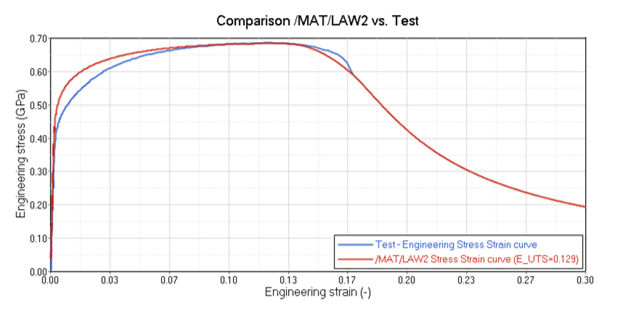
Figure 6. Comparison of Results using /MAT/LAW2 and the Test

/MAT/LAW36: Elasto-plastic Material Law using a Tabulated Input Function

Since tensile test data is available, a more accurate method is to use that data in material LAW36. The first step is to take the test data and calculate the true stress versus true plastic strain curve by using Equation 4 and Equation 7.


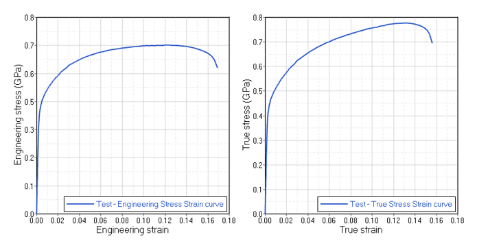
Figure 7. Engineering Stress vs Strain Compared to True Stress-Strain, Experimental Data

The necking point is where the slope of the engineering stress-strain curve becomes zero. All values after the necking point can not be used for creating the material curve for /MAT/LAW36 and can be removed from the data and disregarded. Values after the necking point must be extrapolated to a strain larger than failure for the material. The necking point occurs at the engineering strain at the ultimate tensile stress = 0.129. After this point, the curve was linearly extrapolated to 100% plastic strain as shown in Figure 8.

Next, the true stress versus true plastic strain is calculated using Equation 8.


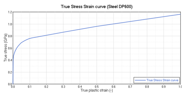
Figure 8. True Stress versus True Plastic Strain Curve Extrapolated to 100%
Using the curve in Figure 8 as input in LAW36, the simulation results perfectly match the test curve between yield point and the necking point, as shown in Figure 9. The post necking behavior depends on the method used to extrapolate the true stress versus true plastic strain data after necking.


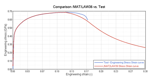
Figure 9. Comparison of the Simulation Results of the Tensile Test with /MAT/LAW36 versus Test

/FAIL/BIQUAD: Simplified Nonlinear Strain-based Failure Criteria with Linear Damage Accumulation

In some elasto-plastic material models, a single plastic strain at failure can be input to model material failure. The element is deleted when the plastic strain reaches a user-defined value ε p m a x .

The main disadvantage of using this approach is the element is deleted when the plastic strain is reached no matter the stress state. There is no difference between failure in tension or compression. Metals usually show different strains at failure for the different states of stress. Especially in the case of compression, the failure strain is usually much higher than for tension. To overcome this limitation, /FAIL/BIQUAD is used instead of the simple maximum equivalent plastic strain that can be defined in the material input. With a few simple inputs, /FAIL/BIQUAD creates a nonlinear plastic strain at failure as a function of stress triaxality.
  • /MAT/LAW2 with /FAIL/BIQUAD
    When the default high strength steel (HSS) values (M_flag =2) included in /FAIL/BIQUAD are used, the simulation shows failure before the test. To better match the test, the /FAIL/BIQUAD uniaxial tension plastic strain at failure value (c3) is increased from 0.5 to 0.75. Figure 10 shows the results for both simulation cases.


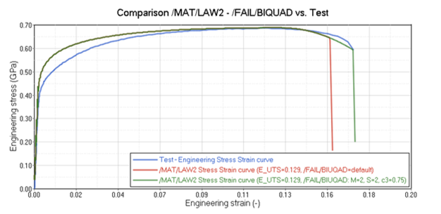
    Figure 10. Comparison of Simulation Results of Tensile Test: /MAT/LAW2 with /FAIL/BIQUAD versus Test
  • /MAT/LAW36 with /FAIL/BIQUAD
    Similar to the LAW2 simulation, the /FAIL/BIQUAD uniaxial tension plastic strain at failure value (c3) is increased from 0.5 to 0.9 so that the failure point in the simulation matches the test.


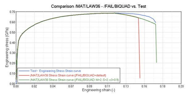
    Figure 11. Comparison of Simulation Results of Tensile Test: /MAT/LAW36 with /FAIL/BIQUAD versus Test

Conclusion

In the first part of the example, a method was introduced to characterize and validate the most commonly used Radioss material laws. The /MAT/LAW2 (PLAS_JOHNS) material was used with a few material parameters to represent the material. The /MAT/LAW36 (PLAS_TAB) material was used with experimental data of a tensile test for a more accurate simulation. The use of "engineering” and "true” stress-strain curves was pointed out.

To describe the failure behavior in tension and compression a simplified nonlinear strain-based failure criterion with linear damage accumulation (/FAIL/BIQUAD) was used to better fit the experimental response.