RD-E: 5501 Fan Blade Rotation Initialization
The /LOAD/CENTRI option in Radioss is used to create the centrifugal force field on fan blades.
In a second Engine file an initial velocity is applied to the model and a /SENSOR is used to deactivate the /LOAD/CENTRI force and apply an imposed velocity to the blades center of rotation.
Options and Keywords Used
- Centrifugal force pre-load in rotating structures
- Rotational velocity about an axis
- Sensor activation
- Implicit followed by Explicit simulations
- Implicit simulation options (Implicit Solution)
- Centrifugal force field (/LOAD/CENTRI)
- Rotational velocity about an axis (/INIV/AXIS/Z/1)
- Load activation and deactivation (/SENSOR/TIME, /SENSOR/NOT)
- Boundary Condition removal in Engine file (/BCSR)
- Johnson-Cook failure model (/FAIL/JOHNSON)
The centrifugal force field is applied to the blades using the /LOAD/CENTRI option with a linear ramp function with a maximum value of 104.72 . Since you want to obtain a steady-state rotation condition, use /LOAD/CENTRI option Ivar=1, the variation of velocity is not taken into account.
When the second Engine file starts, an initial and constant imposed rotational velocity of 104.72 is applied to the blades. The imposed velocity (/IMPVEL) is activated using a time activated sensor (/SENSOR/TIME) at t=0.1 seconds. A sensor TYPE=NOT (/SENSOR/NOT) is used to turn off the centrifugal force when the imposed velocity is turned on. The /SENSOR/NOT activation state is opposite of the sensor it references and; thus, it will be on from time = 0 – 0.1 seconds.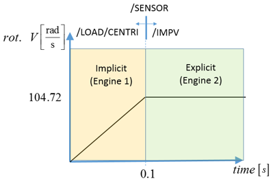
Figure 1.To keep the implicit solution in static equilibrium, a fully-constrained boundary condition (/BCS) is used on the main node of the rigid body that connects the base nodes of the blades. This fully-constrained boundary condition is removed in a second Engine file when rotation begins.
| Command | Comments | |
|---|---|---|
| Print Info | /PRINT/-1 /IMPL/PRINT/NONL/-1 |
Printout frequency for nonlinear computation. |
| Linear Solver Method | /IMPL/SOLVER/3 | N=3 for direct solver. Uses BCS in SMP
and MUMPS in SPMD. Linear solver is also used in nonlinear iteration. It is used to resolve in each iteration of nonlinear cycle. |
| Nonlinear Solver Method | /IMPL/NONLIN/1 0, 12, 0.01, 0.01
|
N=1 (default) used with Modified Newton
method. Itol=12: use relative residual in energy (Ioli=0.01 as tolerance) and in force (Iolj=0.01 as tolerance) as termination criteria. |
| /IMPL/LSEARCH/1 20, 1.0E-03 |
Line search methods for nonlinear
analysis. N=1: use standard line-searches minimizing energy residual MAX_ls=20 (default): maximum line search iteration number is 20 TOL_ls=1e-3 (default): tolerance for line search iteration is 1e-3 |
|
| Time Step | /IMPL/DTINI 0.01E+00 |
Use to define initial time step for nonlinear implicit analysis. |
| /IMPL/DT/STOP
0.01E-04,0.03E+00 |
Implicit analysis will be stopped if DT_min=0.01e-4, and once DT_max=0.03 is reached, computation will continue with this maximum time step. | |
| /IMPL/DT/2 6,0.00E+00,20,0.67E+00,0.11E+01 |
Implicit time step control . Desired convergence iteration number is 6 (default). Set maximum convergence iteration number 20 (default). Decreasing time step factor set to 0.67 (default). Max. scale factor for increasing the time step set to 1.1 (default). |
# initialize the explicit rotation
/RUN/fbo_case/2
            0.200
…
# apply initial rotational velocity
/INIV/AXIS/Z/1
0
0 0 0 104.72
1 3650
# remove z rotation boundary condition on main node of rigid body (node ID 5)
/BCSR/ROT/Z
         5
Input Files
- <install_directory>/hwsolvers/demos/radioss/example/55_Fan_Blade_Out_FBO/1_Initialize_rotation_stress/*
Model Description
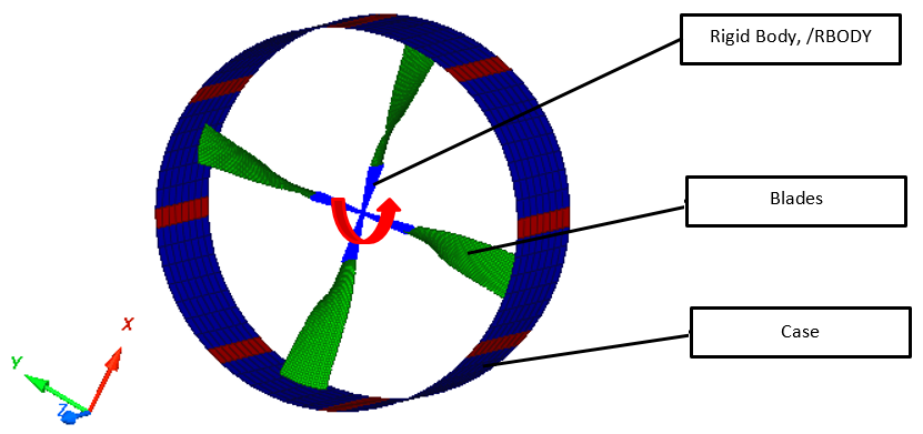
Figure 2. Blades with Case
Units: mm, s, Mg, N, and MPa
- Blade Titanium Material Properties
- Density
- Young's modulus
- 113400
- Poisson's ratio
- 0.342
- Yield stress
- 1098
- Plastic hardening parameter
- 1092
- Plastic hardening exponent
- 0.93
- Case Steel Material Properties
- Density
- Young's modulus
- 210000
- Poisson's ratio
- 0.3
- Yield stress
- 200
- Plastic hardening parameter
- 450
- Plastic hardening exponent
- 0.5
- Maximum stress
- 425
- Blade Center constrained all directions, except Rz
- Imposed Rotational Speed = 1000 = 104.72
- Edges of case are fully constrained in X, Y, Z directions
Model Method
The purpose of the analysis is to initialize the centrifugal force field and stress on the blades from a 1000 RPM rotation. One method to initialize the centrifugal force would be to slowly increase to rotational speed from 0 to 1000 RPM. However, for explicit simulations this can be very time consuming. To reduce the simulation time, the implicit solution method and the /LOAD/CENTRI option in Radioss can be used to create the centrifugal force field. Using a second Engine file, an initial rotational velocity is applied to the blades and a /SENSOR is used to turn off the centrifugal force field and turn on an imposed velocity, (/IMPVEL). Now that the blades are rotating, the stress remains constant which means the blades are in steady-state rotation.
Results
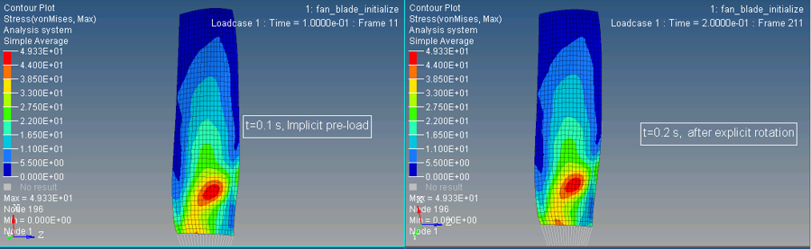
Figure 3. Comparison of Stress after Centrifugal Load in Implicit and Explicit Rotation
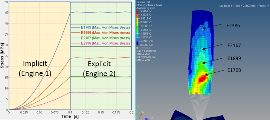
Figure 4. Time History Plot of Element Stress
Conclusion
Now that the force on the blades is correctly applied and the blades are rotating in a steady-state condition, a fan blade out simulation or blade impact by a bird or hailstone could be completed.