RD-E: 1602 IMPLICIT Solver
A dummy is sat down via gravity using the implicit approach (static).
- Unconditional stable scheme
- Large time step
- Treatment of the static problem
Options and Keywords Used
- Shell, brick, beam, spring, and dummy
- Linear and nonlinear static solution by implicit solver
- Symmetric interface (/INTER/TYPE7) and tied interface (/INTER/TYPE2)
- Kelvin-Voigt visco-elastic model (/MAT/LAW35 (FOAM_VISC)) and linear elastic law (/MAT/LAW1 (ELAST))
- Concentrated load (/CLOAD)
- Imposed displacement (/IMPDISP)
- Time step control method for implicit (Implicit Time Step)
- Initial time step for implicit (/IMPL/DTINI)
- Static linear implicit solution (/IMPL/LINEAR)
- Static nonlinear implicit solution (/IMPL/NONLIN)
- Print frequency for implicit (/IMPL/PRINT/LINEAR)
- Implicit solver method (/IMPL/SOLVER)
- Gravity (/GRAV)
Input Files
- Linear_implicit_model
- <install_directory>/hwsolvers/demos/radioss/example/16_Dummy_Positioning/IMPLICIT_solver/Linear/SEAT_IMPL_LIN*
- Nonlinear_implicit_model
- <install_directory>/hwsolvers/demos/radioss/example/16_Dummy_Positioning/IMPLICIT_solver/Nonlinear/
Linear and Nonlinear Analysis
However, the implicit algorithm uses a global resolution which requires convergence for each time step and has low robustness in comparison to the explicit (null pivots, divergence for high nonlinearities, etc.).
- Newmark
- Implicit integration scheme
This scheme is unconditionally stable, the stability condition being independent of the time step choice. See the Radioss Theory Manual for further information about the Newmark scheme.
Radioss has a linear and a nonlinear solver. Only static computations are available and loading should be defined as a monotonous increasing time function for nonlinear analysis.
- Cholesky (direct method, linear solver)
- Preconditioned Conjugate Gradient (linear solver)
- Modified Newton-Raphson method (nonlinear solver)
- No preconditioned
- Diagonal Jacobi
- Incomplete Cholesky
- Stabilized incomplete Cholesky
- Factored Approximate Inverse (by default)
You should define the tolerance and stop criterion for the linear and nonlinear solver (residual).
- Iterations number limit for updating stiffness matrix
- Convergence iterations number for increasing time step
- Convergence iterations number for decreasing time step
- Increase time step factor
- Decrease time step factor
- Minimum time step
- Maximum time step
- Initial time step
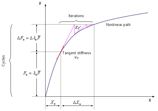
Figure 1. Newton-Raphson Resolution in the Case of Load Control Technique
The modified Newton-Raphson method is based on maintaining the tangent matrix for all iterations and can be combined with the line search acceleration technique for accelerating convergence.
- Displacement norm control
- Arc-length control
An automatic time step control is used.
Static Analysis and Implicit Options
- A static linear computation (loading by gravity)
- A static nonlinear computation (three computations are performed: dummy positioning using an imposed displacement, followed by a concentrated load and a gravity loading).
An adapted modeling methodology is set up for each analysis. Contact with the different interfaces depends on the computations taken into account and then the material can be updated.
The goal for this analysis is to propose a modeling method for different loading cases, with specific input data used in the implicit strategies. The studies by linear implicit and nonlinear implicit using imposed displacement are no longer comparable with results obtained by explicit, due to the different physical approaches. Comparisons are only valid for the positioning by gravity loading.
Model Description
Linear Static Analysis
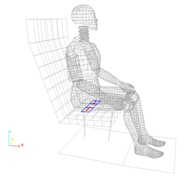
Figure 2. TYPE2 Tied Interface Linear Contact for Dummy/Seat Cushion Modeling
- Material Properties
- Young's modulus
- 0.2
- Poisson's ratio
- 0
- Density
- 4.3 x 10⁻¹¹ k g/l
Model Method
You can select BATOZ formulations for the shell elements and HA8 formulations using 2x2x2 integration points for the brick elements.
- Implicit type
- Static linear
- Linear solver
- Direct Cholesky
- Precondition method
- Factored Approximate Inverse
- Stop criteria
- Relative residual of preconditioned matrix
- Tolerance
- 10-6
- /IMPL/PRINT/LINEAR/-1
- Printout frequency for linear iteration
- /IMPL/SOLVER/3
- Solver method
- 5 0 3 0.0
- /IMPL/LINEAR
- Static linear computation
Results
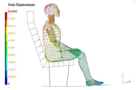
Figure 3. Linear Static Implicit Solution of Gravity Loading (TYPE2 interface is used)
| Explicit Solver - /DYREL | Implicit Solver - Linear | |
|---|---|---|
| Normalized CPU | 170 | 1 |
Nonlinear Static Analysis
Positioning Using an Imposed Displacement
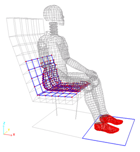
Figure 4. Nonlinear Contact Modeling with Self-impacting TYPE7 Interface
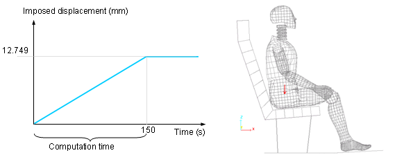
Figure 5. Imposed Displacement Along the Z-axis as a Monotonous Increasing Time Function
- Implicit type
- Static nonlinear
- Nonlinear solver
- Modified Newton
- Stop criteria
- Relative residual in force
- Tolerance
- 0.01
- Update of stiffness matrix
- 5 iterations maximum
- Time step control method
- Arc-length method and "line-search"
- Initial time step
- 5 s
- Minimum time step
- 0.01 s
- Maximum time step
- no
- Desired convergence iteration number
- 6
- Maximum convergence iteration number
- 20
- Decreasing time step factor
- 0.8
- Maximum increasing time step scale factor
- 1.1
- Arc-length
- Automatic computation
- Spring-back option
- no
Implicit parameters are set in the Engine file with the options beginning with /IMPL.
- /IMPL/PRINT/NONLIN/-1
- Printout frequency for nonlinear iteration
- /IMPL/SOLVER/3 5 0 3 0.0
- Solver method (solve Ax=b)
- /IMPL/NONLIN 5 2 0.01
- Static nonlinear computation
- /IMPL/DTINI 1
- Initial time step determines the initial loading increment
- /IMPL/DT/STOP 1e-3 0
- Min-Max values for time step
- /IMPL/DT/2 6.0 20 0.8 1.1
- Time step control metho 2 - Arc-length+Line-search will be used with this method to accelerate and control convergence
Due to the contact problem, the tolerance value (Tol) is set to 10-2 (default = 10-3).
Some options are not compatible with the implicit solver. Refer to Radioss Starter Input for more details about implicit options.
Results
The last animation corresponds to the static solution.
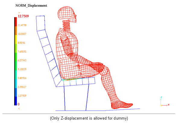
Figure 6. Nonlinear Static Implicit Solution of the Imposed Displacement
| Explicit Solver - /DYREL | Implicit Solver - Nonlinear | |
|---|---|---|
| Normalized CPU | 1.26 | 1 |
| Number of cycles (normalized) | 56704 (1718) | 33 (1) |
Positioning Using a Concentrated Load
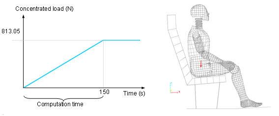
Figure 7. Concentrated Load Along the Z-axis as a Monotonous Increasing Time Function
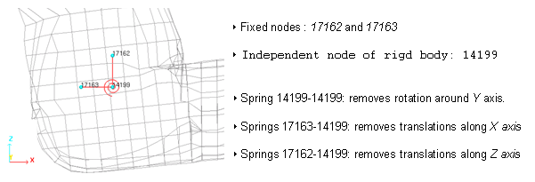
Figure 8. Springs TYPE8 Defined for Removing Rigid Body Modes during Implicit Computation
- Linear elastic behavior
- Mass = 1g
- Inertia = 0.001
- Translational stiffness: TX = 1 N/mm
TY = 1 N/mm
TZ = 1 N/mm
- Rotational stiffness: RX = 100 Mg.mm2/(s2.rad)
RY = 100 Mg.mm2/(s2.rad)
RZ = 100 Mg.mm2/(s2.rad)
Implicit options are the same as the previous implicit problem; except for the initial time step is set to: 2s.
Results
| Explicit Solver - /DYREL | Implicit Solver - Nonlinear | |
|---|---|---|
| Normalized CPU | 3.07 | 1 |
| Number of cycles (normalized) | 56704 (1090) | 52 (1) |
| Z - displacement (main node dummy) | -12.75 mm | -12.49 mm |
Positioning Using Gravity Loading
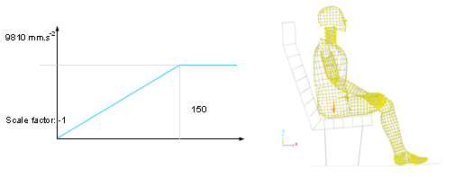
Figure 9. Gravity Loading as a Monotonous Increasing Time Function
Implicit options are the same as the previous implicit problem (initial time step is set to: 2s).
Results
| Explicit solver - /DYREL | Implicit solver - Nonlinear | |
|---|---|---|
| Normalized CPU | 2.53 | 1 |
| Number of cycles (normalized) | 56704 (1090) | 52 (1) |
| Z - displacement (main node dummy) | -12.75 mm | -12.42 mm |
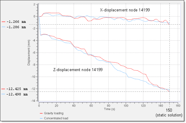
Figure 10. Convergence results of the X- and Z-displacement of main node 14199 (rigid body dummy). for the implicit models using gravity loading and concentrated load
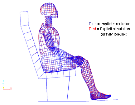
Figure 11. Final dummy position obtained using IMPLICIT (model using gravity loading) . (and EXPLICIT model with gravity loading and kinetic relaxation)
Conclusion
This example brings awareness to the use of the Radioss implicit solver in resolving quasi-static problems. On the other hand, it illustrates different convergence acceleration techniques when an explicit solver is applied to the quasi-static problems. The advantages and drawbacks of the methods are compared.