RD-E: 1601 EXPLICIT Solver

A dummy is sat down via gravity using the quasi-static load treatment.

The topic of this study concerns quasi-static load treatment using kinetic relaxation, dynamic relaxation and Rayleigh damping. The explicit solutions provided by the three different approaches will be compared and analyzed.

Options and Keywords Used

The goal is to set the body on the seat using a quasi-static approach in order to obtain static equilibrium. The positioning phase is not included in this study. Thus, all nodes of the dummy are placed in a global rigid body in order to maintain the dummy's initial configuration.

In order to save the CPU, a second global rigid body includes parts of the seat and the floor; except for the seat cushion parts, which will only have active elements during simulation.

rad_ex_fig_16-6
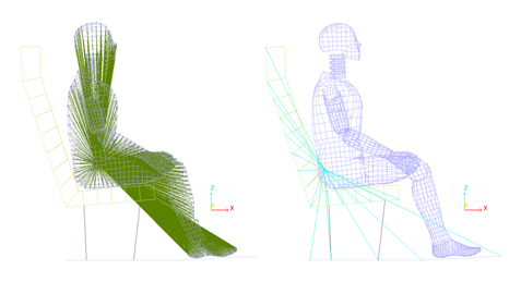
Figure 1. Set up of Both Rigid Bodies

When the ICoG flag is set to 1 for the rigid body of the seat, the center of gravity is computed using the main and secondary node coordinates, and the main node is moved to the center of gravity, where mass and inertia are placed.

When the ICoG flag is set to 3 for the rigid body of the dummy, the center of gravity is set at the main node coordinates defined by you. The added masses and added inertia are transmitted to the main node coordinates.

The main node coordinates and skew are extracted from the pelvis part of the original rigid body.

Gravity is applied to all nodes of the model. A function defines gravity acceleration in the z direction versus time. Gravity is activated by /GRAV in the Starter file (*_0000.rad).

rad_ex_fig_16-7
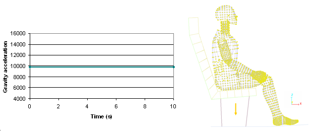
Figure 2. Input Gravity Function (-9810 mm/s-2) and Nodes Selection (yellow)
The six rigid body modes of the seat are removed by completely fixing the rigid body main node attached to the seat. In order to limit the out-of-plane vibrations, the main node of the dummy's rigid body is fixed in translation along the Y axis.

rad_ex_fig_16-8
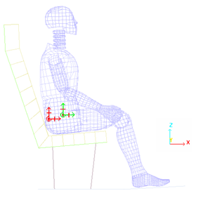
Figure 3. Boundary Conditions on the Rigid Bodies' Main Nodes

Static analysis: quasi-static treatment of gravity loading up to static equilibrium.

The explicit time integration scheme starts with nodal acceleration computation. It is efficient for simulating dynamic loading. However, a quasi-static simulation via a dynamic resolution method needs to minimize the dynamic effects in order to converge towards static equilibrium. This usually describes the pre-loading case prior to dynamic analysis. Thus, the quasi-static solution of gravity loading on the model is the steady-state part of the transient response.

To reduce the dynamic effect, three options are available in the Engine file:
  • Kinetic relaxation (/KEREL)
  • Dynamic relaxation (/DYREL)
  • Rayleigh damping (/DAMP)

Kinetic Relaxation Method

All velocities are set to zero each time the kinetic energy reaches a maximum value. This option is activated in the Engine file using /KEREL (input is not required).

rad_ex_fig_16-9
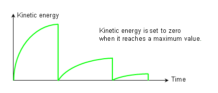
Figure 4. Kinetic Relaxation Method with /KEREL (also named energy discrete relaxation)

Dynamic Relaxation Method

Dynamic loading is damped by introducing a diagonal damping matrix, proportional to mass matrix, in the dynamic equation:(1) [ M ] { u ¨ } + [ C ] { u ˙ } + [ K ] { u } = F [ C ] = 2 β T [ M ] MathType@MTEF@5@5@+= feaagKart1ev2aaatCvAUfeBSjuyZL2yd9gzLbvyNv2CaerbuLwBLn hiov2DGi1BTfMBaeXatLxBI9gBaerbd9wDYLwzYbItLDharqqtubsr 4rNCHbGeaGqiVu0Je9sqqrpepC0xbbL8F4rqqrFfpeea0xe9Lq=Jc9 vqaqpepm0xbba9pwe9Q8fs0=yqaqpepae9pg0FirpepeKkFr0xfr=x fr=xb9adbaqaaeGaciGaaiaabeqaamaabaabaaGceaqabeaadaWada qaaiaad2eaaiaawUfacaGLDbaadaGadaqaaiqadwhagaWaaaGaay5E aiaaw2haaiabgUcaRmaadmaabaGaam4qaaGaay5waiaaw2faamaacm aabaGabmyDayaacaaacaGL7bGaayzFaaGaey4kaSYaamWaaeaacaWG lbaacaGLBbGaayzxaaWaaiWaaeaacaWG1baacaGL7bGaayzFaaGaey ypa0JaamOraaqaamaadmaabaGaam4qaaGaay5waiaaw2faaiabg2da 9maalaaabaGaaGOmaiabek7aIbqaaiaadsfaaaWaamWaaeaacaWGnb aacaGLBbGaayzxaaaaaaa@5530@
With,
β
Relaxation value (recommended default value 1)
T
The period to be damped (less than or equal to the highest period of the system)
Thus, a viscous stress tensor is added to the stress tensor:(2) σ ij viscous =( λ+2μ ) ε ˙ kk δ ij +2μ ε ˙ ij MathType@MTEF@5@5@+= feaagKart1ev2aaatCvAUfeBSjuyZL2yd9gzLbvyNv2CaerbuLwBLn hiov2DGi1BTfMBaeXatLxBI9gBaerbd9wDYLwzYbItLDharqqtubsr 4rNCHbGeaGqiVu0Je9sqqrpepC0xbbL8F4rqqrFfpeea0xe9Lq=Jc9 vqaqpepm0xbba9pwe9Q8fs0=yqaqpepae9pg0FirpepeKkFr0xfr=x fr=xb9adbaqaaeGaciGaaiaabeqaamaabaabaaGcbaGaeq4Wdm3aa0 baaSqaaiaadMgacaWGQbaabaGaamODaiaadMgacaWGZbGaam4yaiaa d+gacaWG1bGaam4Caaaakiabg2da9maabmaabaGaeq4UdWMaey4kaS IaaGOmaiabeY7aTbGaayjkaiaawMcaaiqbew7aLzaacaWaaSbaaSqa aiaadUgacaWGRbaabeaakiabes7aKnaaBaaaleaacaWGPbGaamOAaa qabaGccqGHRaWkcaaIYaGaeqiVd0MafqyTduMbaiaadaWgaaWcbaGa amyAaiaadQgaaeqaaaaa@569E@
Using an explicit code, application of the dashpot force reduces the velocity equation modification:(3) V t + Δ t / 2 = V t Δ t / 2 + γ t Δ t MathType@MTEF@5@5@+= feaagKart1ev2aaatCvAUfeBSjuyZL2yd9gzLbvyNv2CaerbwvMCKf MBHbqefqvATv2CG4uz3bIuV1wyUbqedmvETj2BSbqefm0B1jxALjhi ov2DaebbnrfifHhDYfgasaacH8srps0lbbf9q8WrFfeuY=Hhbbf9v8 qqaqFr0xc9pk0xbba9q8WqFfea0=yr0RYxir=Jbba9q8aq0=yq=He9 q8qqQ8frFve9Fve9Ff0dmeaacaGacmGadaWaaiqacaabaiaafaaake aacaWGwbWaaSbaaSqaaiaadshacqGHRaWkcqqHuoarcaWG0bGaai4l aiaaikdaaeqaaOGaeyypa0JaamOvamaaBaaaleaacaWG0bGaeyOeI0 IaeuiLdqKaamiDaiaac+cacaaIYaaabeaakiabgUcaRiabeo7aNnaa BaaaleaacaWG0baabeaakiabfs5aejaadshaaaa@4D73@ (4) V t + Δ t / 2 = ( 1 2 ω ) V t Δ t / 2 + ( 1 ω ) γ t Δ t MathType@MTEF@5@5@+= feaagKart1ev2aaatCvAUfeBSjuyZL2yd9gzLbvyNv2CaerbwvMCKf MBHbqefqvATv2CG4uz3bIuV1wyUbqedmvETj2BSbqefm0B1jxALjhi ov2DaebbnrfifHhDYfgasaacH8srps0lbbf9q8WrFfeuY=Hhbbf9v8 qqaqFr0xc9pk0xbba9q8WqFfea0=yr0RYxir=Jbba9q8aq0=yq=He9 q8qqQ8frFve9Fve9Ff0dmeaacaGacmGadaWaaiqacaabaiaafaaake aacaWGwbWaaSbaaSqaaiaadshacqGHRaWkcqqHuoarcaWG0bGaai4l aiaaikdaaeqaaOGaeyypa0ZaaeWaaeaacaaIXaGaeyOeI0IaaGOmai abeM8a3bGaayjkaiaawMcaaiaadAfadaWgaaWcbaGaamiDaiabgkHi Tiabfs5aejaadshacaGGVaGaaGOmaaqabaGccqGHRaWkdaqadaqaai aaigdacqGHsislcqaHjpWDaiaawIcacaGLPaaacqaHZoWzdaWgaaWc baGaamiDaaqabaGccqqHuoarcaWG0baaaa@582B@

This option is activated in the Engine file (*_0001.rad) using /DYREL (inputs: β and T ).

Rayleigh Damping Method

Dynamic loading is damped by introducing a damping matrix, proportional to the mass and stiffness matrix, in the dynamic equation. This simplified approach will allow you to reduce the global equilibrium equation to n-uncoupled equations by using an orthogonal transformation. This damping is said to be proportionally uncoupled.(5) [ M ] { u ¨ } + [ C ] { u ˙ } + [ K ] { u } = F [ C ] = a [ M ] + β [ M ] MathType@MTEF@5@5@+= feaagKart1ev2aaatCvAUfeBSjuyZL2yd9gzLbvyNv2CaerbuLwBLn hiov2DGi1BTfMBaeXatLxBI9gBaerbd9wDYLwzYbItLDharqqtubsr 4rNCHbGeaGqiVu0Je9sqqrpepC0xbbL8F4rqqrFfpeea0xe9Lq=Jc9 vqaqpepm0xbba9pwe9Q8fs0=yqaqpepae9pg0FirpepeKkFr0xfr=x fr=xb9adbaqaaeGaciGaaiaabeqaamaabaabaaGceaqabeaadaWada qaaiaad2eaaiaawUfacaGLDbaadaGadaqaaiqadwhagaWaaaGaay5E aiaaw2haaiabgUcaRmaadmaabaGaam4qaaGaay5waiaaw2faamaacm aabaGabmyDayaacaaacaGL7bGaayzFaaGaey4kaSYaamWaaeaacaWG lbaacaGLBbGaayzxaaWaaiWaaeaacaWG1baacaGL7bGaayzFaaGaey ypa0JaamOraaqaamaadmaabaGaam4qaaGaay5waiaaw2faaiabg2da 9iaadggadaWadaqaaiaad2eaaiaawUfacaGLDbaacqGHRaWkcqaHYo GydaWadaqaaiaad2eaaiaawUfacaGLDbaaaaaa@5817@

Where, a and β are the pre-defined constants.

The orthogonal transformation using this proportional damping assumption leads to:(6) ξ i = α 2 ω i + β ω i 2 MathType@MTEF@5@5@+= feaagKart1ev2aaatCvAUfeBSjuyZL2yd9gzLbvyNv2CaerbwvMCKf MBHbqefqvATv2CG4uz3bIuV1wyUbqedmvETj2BSbqefm0B1jxALjhi ov2DaebbnrfifHhDYfgasaacH8srps0lbbf9q8WrFfeuY=Hhbbf9v8 qqaqFr0xc9pk0xbba9q8WqFfea0=yr0RYxir=Jbba9q8aq0=yq=He9 q8qqQ8frFve9Fve9Ff0dmeaacaGacmGadaWaaiqacaabaiaafaaake aacqaH+oaEdaWgaaWcbaGaamyAaaqabaGccqGH9aqpdaWcaaqaaiab eg7aHbqaaiaaikdacqaHjpWDdaWgaaWcbaGaamyAaaqabaaaaOGaey 4kaSYaaSaaaeaacqaHYoGycqaHjpWDdaWgaaWcbaGaamyAaaqabaaa keaacaaIYaaaaaaa@4860@
With,
ξ i
The i th being the damping ratio of the system
ω i
The i th being the natural frequency of the system.

rad_ex_fig_16-10
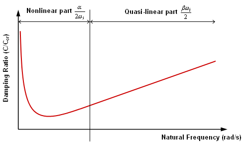
Figure 5. Rayleigh Type Damping
If you have some experimental results, the proportionality factors, a and β are found by evaluating the damping for a pair of the most significant frequencies used. Thus, two equations with two unknown variables are obtained:(7) 2 ζ 1 = a ω 1 + β ω 1 2 ζ 2 = a ω 2 + β ω 2 MathType@MTEF@5@5@+= feaagKart1ev2aaatCvAUfeBSjuyZL2yd9gzLbvyNv2CaerbuLwBLn hiov2DGi1BTfMBaeXatLxBI9gBaerbd9wDYLwzYbItLDharqqtubsr 4rNCHbGeaGqiVu0Je9sqqrpepC0xbbL8F4rqqrFfpeea0xe9Lq=Jc9 vqaqpepm0xbba9pwe9Q8fs0=yqaqpepae9pg0FirpepeKkFr0xfr=x fr=xb9adbaqaaeGaciGaaiaabeqaamaabaabaaGcbaGaaGOmaiabeA 7a6naaBaaaleaacaaIXaaabeaakiabg2da9maalaaabaGaamyyaaqa aiabeM8a3naaBaaaleaacaaIXaaabeaaaaGccqGHRaWkcqaHYoGycq aHjpWDdaWgaaWcbaGaaGymaaqabaGccaaMf8UaaGzbVlaaikdacqaH 2oGEdaWgaaWcbaGaaGOmaaqabaGccqGH9aqpdaWcaaqaaiaadggaae aacqaHjpWDdaWgaaWcbaGaaGOmaaqabaaaaOGaey4kaSIaeqOSdiMa eqyYdC3aaSbaaSqaaiaaikdaaeqaaaaa@53D5@

If several frequencies are available, an average of computed values, a and β may be used.

This model of proportional damping is not recommended for complex structures and does not enable good experimental retiming.

This option is activated in the Engine file (*_0001.rad) using /DAMP (inputs data: a and β ).

Parameters Used

In this example, a and β are set to:
  • First case: a = 10 and β = 10
  • Second case: a = 0 and β = 10
  • Third case: a = 10 and β = 0
  • Fourth case: a = 20 and β = 0
The resulting assumptions are:
First case
[C] = 10[M] + 10[K]
Second case
[C] = 10[K]
Third case
[C] = 10[M]
Fourth case
[C] = 20[M]

Input Files

The input files used in this example include:
Rayleigh_damping
<install_directory>/hwsolvers/demos/radioss/example/16_Dummy_Positioning/EXPLICIT_solver/RAYLEIGH/.../SEAT_RAYLEIGH*
Dynamic_relaxation
<install_directory>/hwsolvers/demos/radioss/example/16_Dummy_Positioning/EXPLICIT_solver/DYREL/SEAT_DYREL*
Kinetic_relaxation
<install_directory>/hwsolvers/demos/radioss/example/16_Dummy_Positioning/EXPLICIT_solver/KEREL/SEAT_KEREL*
Without_damping
<install_directory>/hwsolvers/demos/radioss/example/16_Dummy_Positioning/EXPLICIT_solver/Without_damping/SEAT*

Model Description

The purpose is to position a dummy on a foam seat under the gravity field using a quasi-static approach prior to a possible dynamic crash simulation.

Units: mm, s, ton, N, MPa

rad_ex_fig_16-1
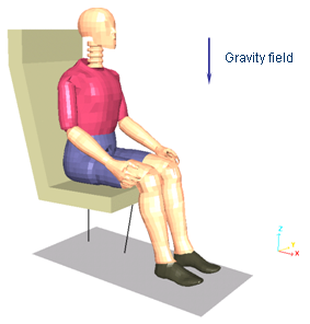
Figure 6. Problem Studied

The dummy weighs 80 kg (173.4 lbs.). The material introduced does not represent the physical case; however, the global weight of the dummy is respected. As the dummy deformation is neglected in this loading phase, simplifying the material characterizations has no incidence on the simulation.

Material for seat brace - both the columns and the floor are made of steel with the following properties (/MAT/LAW1):
Material Properties
Young's modulus
210000 [ MPa ] MathType@MTEF@5@5@+= feaagKart1ev2aqatCvAUfeBSjuyZL2yd9gzLbvyNv2CaerbuLwBLn hiov2DGi1BTfMBaeXatLxBI9gBaerbd9wDYLwzYbItLDharqqtubsr 4rNCHbGeaGqiVu0Je9sqqrpepC0xbbL8F4rqGqFfpeea0xe9vq=Jb9 vqpeea0xd9q8qiYRWxGi6xij=hbba9q8aq0=yq=He9q8qiLsFr0=vr 0=vr0db8meaabaqaciGacaGaaeqabaWaaeaaeaaakeaadaWadaqaai Gac2eacaGGqbGaaiyyaaGaay5waiaaw2faaaaa@3BE6@
Poisson's ratio
0.3
Density
7.8 x 10⁻⁹ Gkg/l
The seat columns have the following characteristics:
Area
2580 mm2
Inertia
IXX = 554975 mm4
IYY = 554975 mm4
IZZ = 937908 mm4
The thickness for the seat back and the floor:
Brace thickness
2 mm
Floor thickness
1 mm
The seat cushion is made of foam which can be described using the generalized Kelvin-Voigt model. The material properties of the foam are:
Material Properties
Young's modulus
0.2 [ MPa ] MathType@MTEF@5@5@+= feaagKart1ev2aqatCvAUfeBSjuyZL2yd9gzLbvyNv2CaerbuLwBLn hiov2DGi1BTfMBaeXatLxBI9gBaerbd9wDYLwzYbItLDharqqtubsr 4rNCHbGeaGqiVu0Je9sqqrpepC0xbbL8F4rqGqFfpeea0xe9vq=Jb9 vqpeea0xd9q8qiYRWxGi6xij=hbba9q8aq0=yq=He9q8qiLsFr0=vr 0=vr0db8meaabaqaciGacaGaaeqabaWaaeaaeaaakeaadaWadaqaai Gac2eacaGGqbGaaiyyaaGaay5waiaaw2faaaaa@3BE6@
Poisson's ratio
0
Density
4.3 x 10⁻¹¹ Gkg/l
E1 and E2
0 [ MPa ] MathType@MTEF@5@5@+= feaagKart1ev2aqatCvAUfeBSjuyZL2yd9gzLbvyNv2CaerbuLwBLn hiov2DGi1BTfMBaeXatLxBI9gBaerbd9wDYLwzYbItLDharqqtubsr 4rNCHbGeaGqiVu0Je9sqqrpepC0xbbL8F4rqGqFfpeea0xe9vq=Jb9 vqpeea0xd9q8qiYRWxGi6xij=hbba9q8aq0=yq=He9q8qiLsFr0=vr 0=vr0db8meaabaqaciGacaGaaeqabaWaaeaaeaaakeaadaWadaqaai Gac2eacaGGqbGaaiyyaaGaay5waiaaw2faaaaa@3BE6@
Tangent modulus
0.25 [ MPa ] MathType@MTEF@5@5@+= feaagKart1ev2aqatCvAUfeBSjuyZL2yd9gzLbvyNv2CaerbuLwBLn hiov2DGi1BTfMBaeXatLxBI9gBaerbd9wDYLwzYbItLDharqqtubsr 4rNCHbGeaGqiVu0Je9sqqrpepC0xbbL8F4rqGqFfpeea0xe9vq=Jb9 vqpeea0xd9q8qiYRWxGi6xij=hbba9q8aq0=yq=He9q8qiLsFr0=vr 0=vr0db8meaabaqaciGacaGaaeqabaWaaeaaeaaakeaadaWadaqaai Gac2eacaGGqbGaaiyyaaGaay5waiaaw2faaaaa@3BE6@
Viscosity in pure shear
10000 MPa/s
C1 = C2 = C3 = 1
Visco-elastic bulk viscosity
Radioss material LAW35 is used. The open cell foam option is not active (Iflag = 0) and the pressure is read using the following input curve:
Table 1. Pressure versus Compression Curve
Compression μ -100000 -10 0 3000 209000 210000
Pressure -1000 -1000 0 7.633 7.633 18.5

Visco-elastic Foam Material Law (/MAT/LAW35)

Based on the Navier equation, LAW35 describes materials using visco-elastic behavior. The effect of the air enclosed is taken into account via a separate pressure versus compression function. Relaxation and creep can be modeled.

The schematic model in Figure 7 describes the generalized Kelvin-Voigt model where a time-dependent spring working in parallel with a Navier dashpot is put in a series with a nonlinear rate-dependent spring.

rad_ex_fig_16-2
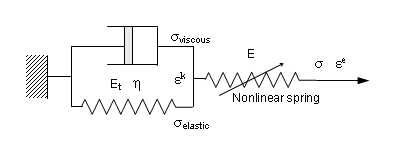
Figure 7. Generalized Kelvin-Voigt Model - LAW35
Two pressure computations are available in Radioss for foam having no open cells. The expression used by default is:(8) d P d t = C 1 K ε ˙ k k C 2 [ K + K t 3 λ + 2 η σ k k ] + C 3 [ K ˙ K t 3 λ + 2 η 0 ε k k ] MathType@MTEF@5@5@+= feaagKart1ev2aaatCvAUfeBSjuyZL2yd9gzLbvyNv2CaerbuLwBLn hiov2DGi1BTfMBaeXatLxBI9gBaerbd9wDYLwzYbItLDharqqtubsr 4rNCHbGeaGqiVu0Je9sqqrpepC0xbbL8F4rqqrFfpeea0xe9Lq=Jc9 vqaqpepm0xbba9pwe9Q8fs0=yqaqpepae9pg0FirpepeKkFr0xfr=x fr=xb9adbaqaaeGaciGaaiaabeqaamaabaabaaGcbaWaaSaaaeaaca WGKbGaamiuaaqaaiaadsgacaWG0baaaiabg2da9iaadoeadaWgaaWc baGaaGymaaqabaGccaWGlbGafqyTduMbaiaadaWgaaWcbaGaam4Aai aadUgaaeqaaOGaeyOeI0Iaam4qamaaBaaaleaacaaIYaaabeaakmaa dmaabaWaaSaaaeaacaWGlbGaey4kaSIaam4samaaBaaaleaacaWG0b aabeaaaOqaaiaaiodacqaH7oaBcqGHRaWkcaaIYaGaeq4TdGgaaiab eo8aZnaaBaaaleaacaWGRbGaam4AaaqabaaakiaawUfacaGLDbaacq GHRaWkcaWGdbWaaSbaaSqaaiaaiodaaeqaaOWaamWaaeaadaWcaaqa aiqadUeagaGaaiaadUeadaWgaaWcbaGaamiDaaqabaaakeaacaaIZa Gaeq4UdWMaey4kaSIaaGOmaiabeE7aOnaaBaaaleaacaaIWaaabeaa aaGccqaH1oqzdaWgaaWcbaGaam4AaiaadUgaaeqaaaGccaGLBbGaay zxaaaaaa@64C8@

Refer to the Radioss Theory Manual for explanation of coefficients.

Pressure may also be computed using the pressure versus compression curve defined by you. The compression, μ is defined as:(9) μ = ρ ρ 0 1 MathType@MTEF@5@5@+= feaagKart1ev2aaatCvAUfeBSjuyZL2yd9gzLbvyNv2CaerbwvMCKf MBHbqefqvATv2CG4uz3bIuV1wyUbqedmvETj2BSbqefm0B1jxALjhi ov2DaebbnrfifHhDYfgasaacH8srps0lbbf9q8WrFfeuY=Hhbbf9v8 qqaqFr0xc9pk0xbba9q8WqFfea0=yr0RYxir=Jbba9q8aq0=yq=He9 q8qqQ8frFve9Fve9Ff0dmeaacaGacmGadaWaaiqacaabaiaafaaake aacqaH8oqBcqGH9aqpdaWcaaqaaiabeg8aYbqaaiabeg8aYnaaBaaa leaacaaIWaaabeaaaaGccqGHsislcaaIXaaaaa@41BB@
Where,
ρ
Density at a time t
ρ 0
Initial density

Model Method

The model consists of two subsets:
  • a dummy composed of 38 parts (limbs and joints).
  • a seat comprised of six parts (foam seat back, foam seat cushion, seat back brace, seat bottom brace, seat columns and the floor).

rad_ex_fig_16-3-4
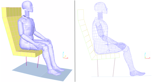
Figure 8. Left: Model Mesh (Perspective view - Shaded display); Right: Model Mesh (Profile view - Edges display)
The seat cushion is meshed with 70 brick elements defined by general TYPE14 solid property.
Quadratic bulk viscosity
1.1
Linear bulk viscosity
0.05
Hourglass viscosity coefficient
0.1

The dummy and seat brace are modeled with shell elements, divided into 4871 4-node shells and 203 3-node shells (Dummy: 5004 shells and seat: 70 shells).

With a dummy in the model, the /DEL/SHELL/1 option should be activated in the Engine file to avoid a small time step, due to the low density of material defining the dummy envelope.
Shell Properties
Belytschko hourglass formulation
Hourglass TYPE4, Ishell = 4
Membrane hourglass coefficients
0.01 (default value)
Out-of-plane hourglass
0.01 (default value)
Rotation hourglass coefficient
0.01 (default value)
Contacts between the dummy and the seat cushion, as well as between the foot and the floor, use TYPE7 interface models with the penalty method. Additionally, symmetrical contact between the body and seat is achieved by creating two complementary interfaces, as:
First interface
Dummy parts
Secondary nodes
Seat
Main surface
Second interface
Dummy parts
Main surface
Seat
Secondary nodes

rad_ex_fig_16-5
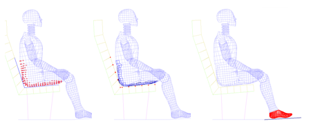
Figure 9. Contacts Modeling with TYPE7 Symmetrical Interface

The gap between the symmetrical interfaces is equal to 5 mm, while a gap of 0.5 mm is set for the other interface.

The TYPE7 interface allows sliding to occur between surfaces. A Coulomb friction can be introduced; in addition, a critical viscous damping coefficient can be defined to damp sliding.
Symmetric Interface Properties
Coulomb friction (Fric flag)
0.3
Critical damping coefficient (Visc flag)
0.05
Scale factor for stiffness (Stfac flag)
1
Sorting factor (Bumult flag)
0.20

Refer to the Radioss Theory Manual and Starter Input for further information about the definition of the TYPE7 interface.

Results

Curve and Animation Results Obtained using Kinetic Relaxation: /KEREL


rad_ex_fig_16-11
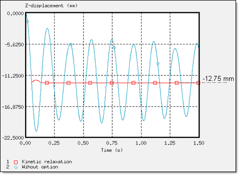
Figure 10. Z-displacement of the Rigid Body's Main Node on Dummy (node 14199)

rad_ex_fig_16-12
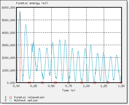
Figure 11. Kinetic Energy of Global Model

Results Obtained using Dynamic Relaxation: /DYREL


rad_ex_fig-16-13
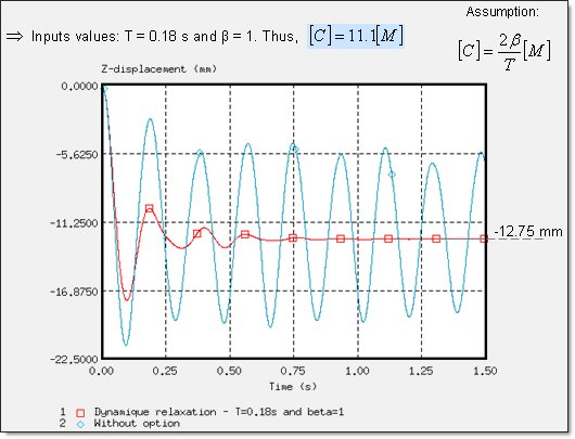
Figure 12. Z-displacement of the Rigid Body's Main Node on Dummy (node 14199)

rad_ex_fig_16-14
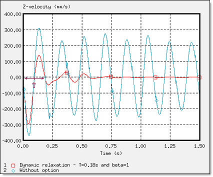
Figure 13. Z-velocity of the Rigid Body's Main Node on Dummy (node 14199)

The period T to be damped is estimated from the velocity curves (highest period).

Results Obtained using Rayleigh Damping: /DAMP


rad_ex_fig_16-15
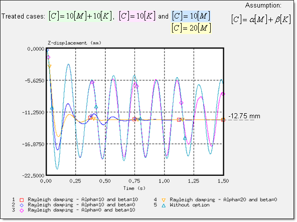
Figure 14. Z-displacement of the Rigid Body's Main Node on Dummy (node 14199)

rad_ex_fig_16-16
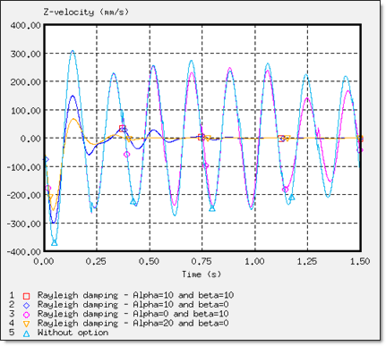
Figure 15. Z-velocity of Rigid Body's Main Node on Dummy (node 14199)

Comparison of the Different Approaches


rad_ex_16-17
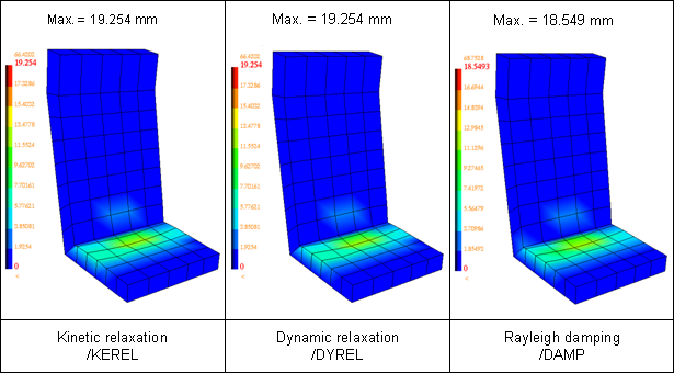
Figure 16. Comparison of the Nodal Displacements' Display on the Seat at Time t = 1.48 s

rad_ex_fig_16-18
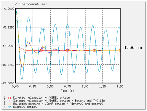
Figure 17. Comparison of Damping on Displacement Obtained using the Three Static Approaches. (Z-displacement of the rigid body's main node on dummy: node 14199)

Conclusion

It is undeniable that the damping methods used to converge towards static equilibrium provide accurate results, especially in the case of this problem where the low rigidity of the seat caused very little quenched oscillations.

The kinetic relaxation introduced in /KEREL, was relatively effective having a swift convergence of the solution towards a static solution, in addition to being easy to use since no input is required. Stability was obtained at 0.137 s.

The /DYREL and /DAMP options are based on viscous damping conducted for the same response, with convergence in three oscillations. Stability was obtained at 0.75 s. Furthermore, dynamic relaxation and the Rayleigh damping methods are basically equivalent in this problem, due to the low stiffness of the seat cushion (Young's modulus is equal to 0.2 [ MPa ] MathType@MTEF@5@5@+= feaagKart1ev2aqatCvAUfeBSjuyZL2yd9gzLbvyNv2CaerbuLwBLn hiov2DGi1BTfMBaeXatLxBI9gBaerbd9wDYLwzYbItLDharqqtubsr 4rNCHbGeaGqiVu0Je9sqqrpepC0xbbL8F4rqGqFfpeea0xe9vq=Jb9 vqpeea0xd9q8qiYRWxGi6xij=hbba9q8aq0=yq=He9q8qiLsFr0=vr 0=vr0db8meaabaqaciGacaGaaeqabaWaaeaaeaaakeaadaWadaqaai Gac2eacaGGqbGaaiyyaaGaay5waiaaw2faaaaa@3BE6@ ), which breaks the balance between the mass and the weight stiffness in the Rayleigh assumption. Moreover, the boundary conditions and the loading applied on the model lead to a problem described using a predominant natural frequency. Thus, only one parameter, a is needed to describe this physical behavior, which reverts back to the dynamic relaxation assumption.

Using β =1 and T =0.18s for dynamic relaxation and β =10 for Rayleigh damping, you achieve:
  • Dynamic relaxation:

    [ C ] = 2 β T [ M ] = 11.1 [ M ] MathType@MTEF@5@5@+= feaagKart1ev2aaatCvAUfeBSjuyZL2yd9gzLbvyNv2CaerbwvMCKf MBHbqefqvATv2CG4uz3bIuV1wyUbqedmvETj2BSbqefm0B1jxALjhi ov2DaebbnrfifHhDYfgasaacH8srps0lbbf9q8WrFfeuY=Hhbbf9v8 qqaqFr0xc9pk0xbba9q8WqFfea0=yr0RYxir=Jbba9q8aq0=yq=He9 q8qqQ8frFve9Fve9Ff0dmeaacaGacmGadaWaaiqacaabaiaafaaake aadaWadaqaaiaadoeaaiaawUfacaGLDbaacqGH9aqpdaWcaaqaaiaa ikdacqaHYoGyaeaacaWGubaaamaadmaabaGaamytaaGaay5waiaaw2 faaiabg2da9iaaigdacaaIXaGaaiOlaiaaigdadaWadaqaaiaad2ea aiaawUfacaGLDbaaaaa@494E@

  • Rayleigh damping:

    [ C ] = α [ M ] + β [ K ] α [ M ]

    10[M]

The approaches available in Radioss provided after convergence a single solution, namely displacement of the dummy by -12.66 mm along the Z-axis and an identical deformation of the seat cushion.