/MAT/LAW76 (SAMP)

Block Format Keyword This law describes a semi-analytical elasto-plastic material using user-defined functions for the work-hardening portion for tension, compression and shear (stress as function of strain).

Format

(1)	(2)	(3)	(4)	(5)	(6)	(7)	(9)
/MAT/LAW76/`mat_ID`/`unit_ID` or /MAT/SAMP/`mat_ID`/`unit_ID`
`mat_title`
$ρ_{i}$
`E`		$ν$
`tab_ID`_t	`tab_ID`_c	`tab_ID`_s
`Fscale`_t		`Fscale`_c		`Fscale`_s			`XFAC`
$ν_{p}$		`fct_ID`_pr	`Fscale`_pr		`F`_smooth	`F`_cut
$ε_{p}^{f}$		$ε_{p}^{r}$
`fct_ID`₁			`Fscale`₁
`I`_form	`IQUAD`	`ICONV`

Definitions

Field	Contents	SI Unit Example
`mat_ID`	Material identifier. (Integer, maximum 10 digits)
`unit_ID`	Unit Identifier. (Integer, maximum 10 digits)
`mat_title`	Material title. (Character, maximum 100 characters)
$ρ_{i}$	Initial density. (Real)	$[\frac{kg}{m^{3}}]$
`E`	Initial Young's modulus. (Real)	$[Pa]$
$ν$	Poisson's ratio. (Real)
`tab_ID`_t	Tension yield stress table identifier (stress vs. plastic tension strain with the possibility of strain rate dependency). (Integer)
`tab_ID`_c	Compression yield stress table identifier (stress vs. plastic compression strain with the possibility of strain rate dependency). (Integer)
`tab_ID`_s	Shear yield stress table identifier (stress vs. plastic shear strain with the possibility of strain rate dependency). (Integer)
`Fscale`_t	Scale factor for ordinate (stress) for `tab_ID`_t. Default = 1.0 (Real)	$[Pa]$
`Fscale`_c	Scale factor for ordinate (stress) for `tab_ID`_c. Default = 1.0 (Real)	$[Pa]$
`Fscale`_s	Scale factor for ordinate (stress) for `tab_ID`_s. Default = 1.0 (Real)	$[Pa]$
`XFAC`	Scale factor for the second entry (strain rate) of the three tables (`tab_ID`_t, `tab_ID`_c, and `tab_ID`_s). 6 Default = 1.0 (Real)
$ν_{p}$	Plastic Poisson's ratio (Real)
`fct_ID`_pr	Plastic Poisson's ratio function identifier ( $ν_{p}$ vs. plastic strain). (Real)
`Fscale`_pr	Scale factor for ordinate ( $ν_{p}$ ) in `fct_ID`_pr. Default = 1.0 (Real)
`F`_smooth	Smooth strain rate option flag. = 0 (Default) No strain rate smoothing. = 1 Strain rate smoothing active. (Integer)
`F`_cut	Cutoff frequency for strain rate filtering. Default = 10³⁰ (Real)	$[Hz]$
$ε_{p}^{f}$	Failure plastic strain (start of element damage). Default = 2e30 (Real)
$ε_{p}^{r}$	Maximum plastic strain (element deleted). Default = 2e30 (Real)
`fct_ID`₁	Damage function identifier (damage vs plastic strain). 2 (Integer)
`Fscale`₁	Scale factor for ordinate for `fct_ID`₁. 2 Default = 1.0 (Real)
`I`_form	Formulation flag. 4 = 0 (Default) No associated formulation. = 1 von Mises associated formulation. (Integer)
`IQUAD`	Yield surface flag. 3 = 0 (Default) Yield surface is linear in the von Mises. = 1 Yield surface is quadratic in the von Mises (recommended). (Integer)
`ICONV`	Convexity condition flag. =0 (Default) No treatment for material stability. = 1 The convexity of yield stress (material stability) is assured. (Integer)

Example (Material)

#RADIOSS STARTER
#---1----|----2----|----3----|----4----|----5----|----6----|----7----|----8----|----9----|---10----|
/UNIT/1
unit for mat
                  kg                  mm                  ms
#---1----|----2----|----3----|----4----|----5----|----6----|----7----|----8----|----9----|---10----|
/MAT/LAW76/1/1
LAW76_Material
#              RHO_I
                1E-6
#                  E                  nu
               100.0                  .3
#  TAB_IDt   TAB_IDc   TAB_IDs 
      1000      1001      1003
#           Fscale_t            Fscale_c            Fscale_s                                    XFAC 
               1.000               1.000               1.000                                   1.000
#               Nu_p  fct_IDpr           Fscale_pr   Fsmooth      Fcut
                 0.5         0                   0         1      1e30
#            EPS_f_p             EPS_r_p 
                   0                   0
#funct_ID1                                Fscale_1
         0
#    IFORM     IQUAD     ICONV
         0         0         1
#---1----|----2----|----3----|----4----|----5----|----6----|----7----|----8----|----9----|---10----|
/TABLE/1/1000
curve_list TENSION strain rates
         2
     10010                        1.0e-4
     10020                           1.0
#---1----|----2----|----3----|----4----|----5----|----6----|----7----|----8----|----9----|---10----|
/FUNCT/10010
eps_vs_sigma funct dt=1.0e-4
              0.0000             .100000
              1.0000             .200000
#---1----|----2----|----3----|----4----|----5----|----6----|----7----|----8----|----9----|---10----|
/FUNCT/10020
eps_vs_sigma funct dt=1.0e-4
              0.0000             .100000
              1.0000             .200000
#---1----|----2----|----3----|----4----|----5----|----6----|----7----|----8----|----9----|---10----|
/TABLE/1/1001
curve_list COMPRESSION strain rates
         2
     10030                        1.0e-4
     10040                           1.0
#---1----|----2----|----3----|----4----|----5----|----6----|----7----|----8----|----9----|---10----|
/FUNCT/10030
eps_vs_sigma funct dt=1.0e-4
              0.0000             .200000
              1.0000             .400000
#---1----|----2----|----3----|----4----|----5----|----6----|----7----|----8----|----9----|---10----|
/FUNCT/10040
eps_vs_sigma funct dt=1.0e-4
              0.0000             .200000
              1.0000             .400000
#---1----|----2----|----3----|----4----|----5----|----6----|----7----|----8----|----9----|---10----|
/TABLE/1/1003
curve_list SHEAR strain rates
         2
     10050                        1.0e-4
     10060                           1.0
#---1----|----2----|----3----|----4----|----5----|----6----|----7----|----8----|----9----|---10----|
/FUNCT/10050
eps_vs_sigma funct dt=1.0e-4
              0.0000             .050000
              0.5000             .060000
              1.0000             .065000
#---1----|----2----|----3----|----4----|----5----|----6----|----7----|----8----|----9----|---10----|
/FUNCT/10060
eps_vs_sigma funct dt=1.0e-4
              0.0000             .050000
              0.5000             .060000
              1.0000             .065000
#---1----|----2----|----3----|----4----|----5----|----6----|----7----|----8----|----9----|---10----|
#ENDDATA
/END

Comments

This material is compatible with shell, thick shell and solid elements.
The material damage can be modeled two ways:
- $ε_{p}^{f}$ (start to damage) and $ε_{p}^{r}$ (element delete)
- Damage function fct_ID₁
  
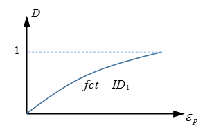
  If damage function fct_ID₁ is used, then $ε_{p}^{f}$ and $ε_{p}^{r}$ will be ignored.
Choice of yield surface:(1)
$f = {\begin{matrix} σ_{V M} - A_{0} - A_{1} P - A_{2} P^{2} I Q U A D = 0 \\ σ_{V M}^{2} - A_{0} - A {}_{1} P - A_{2} P^{2} I Q U A D = 1 \end{matrix}$

Where,(2)
$P = - \frac{σ_{x x} + σ_{y y} + σ_{z z}}{3}$
(3)
$σ_{V M} = \sqrt{\frac{3}{2} [{(σ_{x x} + P)}^{2} + {(σ_{y y} + P)}^{2} + {(σ_{z z} + P)}^{2} + 2 σ_{x y}^{2} + 2 σ_{y z}^{2} + 2 σ_{x z}^{2}]}$

$A_{0}$ , $A_{1}$ and $A_{2}$ coefficients are computed from the hardening curve given for tension, compression and shear.

For von Mises and Drücker-Prager yield surface, IQUAD=0 can be used. However, in some situations, it can be difficult for Radioss to fit the $A_{0}$ , $A_{1}$ and $A_{2}$ coefficients when using IQUAD=0 and an easier fit is obtained by using IQUAD=1.
Choice of plasticity formulation:
- For the no associated plasticity formulation, I_form=0:
  The plastic flow rule function, $g$ , is used to describe plastic strain increment $d ε_{p} = d λ \frac{\partial g}{\partial σ}$ . In this case $\frac{\partial g}{\partial σ}$ is not normal to the yield surface $f$ and $g$ is not associated with the yield surface $f$ .
  
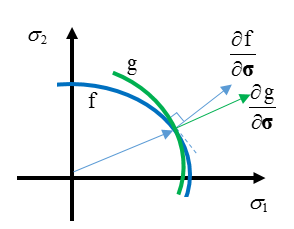
  Figure 1.
  
  The plastic flow rule, $g$ , is given by: (4)
  $g = \sqrt{σ_{V M}^{2} + α P^{2}}$
  
  Materials like soil or rock usually use the no associated plasticity formulation, I_form=0.
- For the associated plasticity: I_form= 1, $g = f$
  In this case, the plastic strain rate is a function of the normal vector of the yield surface $f$ . Materials like metal usually use the associated plasticity formulation.(5)
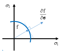
  $d ε_{p} = d λ \frac{\partial f}{\partial σ} = d λ \frac{\partial g}{\partial σ}$
  
  Figure 2.
The convexity condition flag ICONV=1 is used to ensure stability in the material law by making sure the yield surface is convex. The yield surface may be hyperbolic for low shear yield values in tension and compression. In this case there is no unique solution and Radioss will update (increase) the shear yield stress to ensure convexity of the yield surface. Therefore, the shear yield stress may be different from input curve.
The tables should have a maximum dimension equal to 2. The first entry is the plastic strain and the second entry is the strain rate.
User variables USR2, USR3, USR4 are used to output plastic strain components in tension, compression and shear. The output is available both for shells and solids in time history and in animation file.