RD-E: 4601 Lagrange Formulation

This example shows how to simulate the cylinder expansion test and compare the simulation result to experimental data.

Detonation is initiated at the bottom of the explosive. Radial expansion of the cylinder is measured and compared to experimental data.

Options and Keywords Used

Lagrange formulation
Jones-Wilkins-Lee EOS (/MAT/LAW5 (JWL))
Hydrodynamic Johnson-Cook Material (/MAT/LAW4 (HYD_JCOOK))
Gruneisen equation of state (/EOS/GRUNEISEN)
Brick elements
Axisymmetrical analysis (/ANALY)
Solid property (/PROP/TYPE14 (SOLID))
Boundary condition (/BCS)
Detonation plan (/DFS/DETPLAN)
Time history on node (/TH/NODE)

Due to the symmetries of the model, a quarter of the cylinder is modeled. Boundary conditions are set on the yOz plan at x = 0 (Tx = 0) and on the xOz plan at y = 0 (Ty = 0) to simulate the symmetry.

A planar detonation wave is defined at the bottom of the cylinder.

In order to plot the curve of radial expansion, displacements of node n 201 520 at z = 24.48 cm on the outer wall of the copper cylinder are saved in time history. It corresponds to L/D=8 in agreement with experimental protocol.(1)

P_{j w l} = A (1 - \frac{ω}{R_{1} V}) e^{- R_{1} V} + B (1 - \frac{ω}{R_{2} V}) e^{- R_{2} V} + \frac{ω (E + Q)}{V}

A scale factor of 0.5 (on time step for all elements) is used for this type of application.

In solid properties, q_a and q_b default values are used. These values have to be changed depending of the formulation (ALE, Euler).

I_solid is set to 14 for copper solid properties.

Radioss Card (TNT)

#---1----|----2----|----3----|----4----|----5----|----6----|----7----|----8----|----9----|---10----|
/PROP/SOLID/2
TNT
#   Isolid    Ismstr               Icpre  Itetra10     Inpts   Itetra4    Iframe                  dn
         0         0                   0         0         0         0         0                   0
#                q_a                 q_b                   h            LAMBDA_V                MU_V
                   0                   0                   0                   0                   0
#             dt_min   istrain      IHKT
                   0         0         0 
#---1----|----2----|----3----|----4----|----5----|----6----|----7----|----8----|----9----|---10----|

Radioss Card (Copper)

#---1----|----2----|----3----|----4----|----5----|----6----|----7----|----8----|----9----|---10----|
/PROP/SOLID/1
Copper
#   Isolid    Ismstr               Icpre  Itetra10     Inpts   Itetra4    Iframe                  dn
         0         0                   0         0         0         0         0                   0
#                q_a                 q_b                   h            LAMBDA_V                MU_V
                   0                   0                   0                   0                   0
#             dt_min   istrain      IHKT
                   0         0         0 
#---1----|----2----|----3----|----4----|----5----|----6----|----7----|----8----|----9----|---10----|

Input Files

The input files used in this example include:

Cylinder Test: <install_directory>/hwsolvers/demos/radioss/example/46_TNT_Cylinder_Expansion_Test/Lagrange/*

Model Description

A OFHC copper cylinder (1.53cm diameter, 0.26cm thickness, 30.5cm height) is filled with an explosive (TNT). Detonation is initiated at the bottom of the explosive. Radial expansion is measured at a length of 8*D cm.

Since this problem is axisymmetric, only a quarter of the cylinder is modeled.

Units: cm, $μ$ s, g, Mbar

The TNT material uses Jones-Wilkins-Lee Material (/MAT/JWL) and Lagrange formulation with the following characteristics:

Material Properties
Initial density: 1.63
A: 3.7121
B: 0.0323
R₁: 4.15
R₂: 0.95
$ω$: 0.3

Chapman Jouget parameters enable detonation time to compute and burn fraction evolution:

Detonation velocity D: 0.693
Chapman Jouguet pressure P_CJ: 0.21
Detonation energy E₀: 0.07

Radioss Card (TNT)

#---1----|----2----|----3----|----4----|----5----|----6----|----7----|----8----|----9----|---10----|
/MAT/JWL/2
TNT 
#              RHO_I
                1.63
#                  A                   B                  R1                  R2               OMEGA
              3.7121               .0323                4.15                 .95                  .3
#                  D                P_CJ                  E0                Eadd   I_BFRAC     Q_OPT
                .693                 .21                 .07                   0         0         0
#             Tstart               Tstop                   a                   m                   n
                   0                   0                   0                   0                   0				
#                 P0                 Psh              a_unit
                   0                   0                   0
#---1----|----2----|----3----|----4----|----5----|----6----|----7----|----8----|----9----|---10----|

Using Hydrodynamic Johnson-Cook material law (/MAT/LAW4), the copper cylinder material has the following characteristics:

Material Properties
Initial density: 8.96
E-Module: 1.24
Poisson's ratio: 0.35
A: 0.9e^-3
B: 0.292e^-2
N: 0.31
$σ_{\max}$: 0.0066
C: 0.025
${\dot{ε}}_{0}$: 1e^-5
M: 1.09
$ρ_{0} C_{p}$: 3.461e^-3
T_melt: 1656

The Gruneisen equation of state (/EOS/GRUNEISEN) is used for copper with the following characteristics:

Material Properties
C: 0.394
S₁: 1.489
$γ {}_{0}$: 1.97
a: 0.47
E₀: 8.96

Radioss Card (Copper)

#---1----|----2----|----3----|----4----|----5----|----6----|----7----|----8----|----9----|---10----|
/MAT/HYD_JCOOK/1
Copper
#              RHO_I
                8.96
#                E0                  nu
                1.24                 .35
#                 A                   B                   n              epsmax              sigmax
              .9E-03            .292E-02                 .31                   0              0.0066
#              Pmin
              -1.E30
#                 C           EPS_DOT_0                   M               Tmelt                Tmax
             .25E-01              .1E-05                1.09              1656.0                1e30
#              RHOCP                                                          Tr
            3.461E-5                                                           0
/EOS/GRUNEISEN/1
Copper
#                  C                  S1                  S2                  S3
                .394               1.489                   0                   0
#             GAMMA0               ALPHA                  E0               RHO_0
                1.97                 .47                   0                8.96 
#---1----|----2----|----3----|----4----|----5----|----6----|----7----|----8----|----9----|---10----|

Model Method

A 3D mesh is made of brick elements. The element size is approximately of 0.035 cm x 0.035 cm x 0.035 cm.

The mesh is dragged along the z direction (z = 30.5 cm). It is important to have no discontinuity in element volume in order to ensure a good propagation of detonation wave and shock wave.

Results

Curves and Animations

The following diagrams display the pressure and density in the cylinder and the explosive.

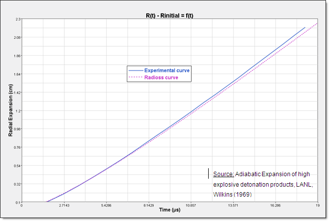
The following diagram shows the comparison between the experimental and simulation measurement of radial expansion.

Conclusion

Good correlation between experimental and simulation results. A thinner meshing could improve the correlation between simulation and experimental curves.

Elapsed time for simulation: t = 11 441 s, 8514 cycles, (4 cpu intel core i7 Q 840 @ 1.87 GHz).

As the model is Lagrangian, the mesh becomes very distorted at the end of the simulation to obtain a proper mesh, it is possible to use the Euler method.