Implicit Example
A shallow cylindrical roof upon which an imposed velocity is applied at its mid-point. Analysis uses an implicit approach.
The purpose of this example is to study a snap-thru problem with a single instability. Thus, a structure that will bend when under a load will be used. The results are compared to a reference solution. 1 An implicit strategy using an arc-length method is illustrated.
Options and Keywords Used
- Implicit solver, time step control by arc-length method
- Static nonlinear analysis
- Stability, snap-thru, and limit load
- T3 Shell
- Boundary conditions (/BCS)
- Implicit options (Implicit Solution)
- Imposed velocity (/IMPVEL)
- Rigid body (/RBODY)
The limit point causes major nonlinearities. Therefore, a static nonlinear analysis is performed using the arc-length displacement strategy. The time step is determined by a displacement norm control. In order to exceed the limit point characterized by a null tangent on the load displacement curve and to describe the increasing and decreasing parts of the nonlinear path, a small time step is required, which is ensured by setting a maximum value.
- Linear Implicit Options
- Linear solver
- Direct solver MUMPS
- Precondition methods
- Factored approximate Inverse
- Maximum iterations number
- System dimension (NDOF)
- Stop criteria
- Relative residual in force
- Tolerance for stop criteria
- Machine precision
- /IMPL/PRINT/NONL/-1
- Printout frequency for nonlinear iteration
- /IMPL/SOLVER/2 5 0 0 0.0
- Solver method (solve Ax=b)
- /IMPL/NONLIN 3 1 0.20e-3
- Static nonlinear computation
- /IMPL/DTINI 10
- Initial time step determines the initial loading increment
- /IMPL/DT/STOP 0.5 10
- Min Max values for time step
- /IMPL/DT/2 6.0 20 0.8 1.05
- Time step control method 2 - Arc-length+Line-search will be used with this method to accelerate and control convergence
Refer to Radioss Starter Input for more details about implicit options.
Input Files
- Implicit solvers
- <install_directory>/hwsolvers/demos/radioss/example/02_Snap-through/Implicit_solver/SNAP_IMP*
Model Descripton
A shallow cylindrical roof, pinned along its straight edges, upon which an imposed velocity is applied at its mid-point.
Units: mm, ms, g, N, MPa
- l
- 254 mm
- R
- 2540 mm
- Shell thickness
- t = 12.7 mm
- 0.1 rad
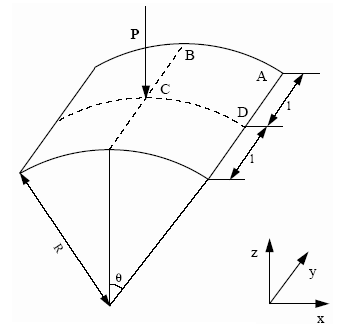
Figure 1. Geometrical Data of the Problem
- Material Properties
- Initial density
- 7.85x10⁻³
- Young's modulus
- 3102.75
- Poisson ratio
- 0.3
Model Method
The modeling problem described in the explicit study remains unchanged.
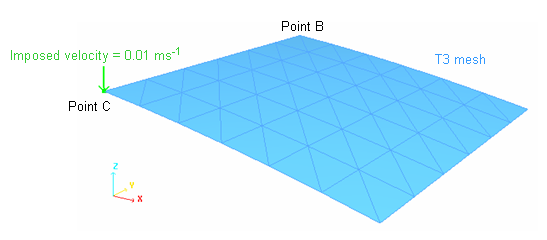
Figure 2. Description of the Problem (one quarter of the shell is modeled)
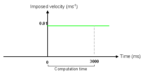
Figure 3. Imposed Velocity Curve
Results
Curves and Animations
Only a quarter of the total load is applied due to the symmetry. Thus, force Fz of the rigid body as indicated in the Time History must be multiplied by 4 in order to obtain force, P.
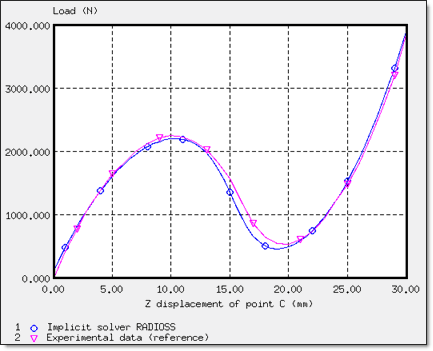
Figure 4. Load P versus Displacement of Point C
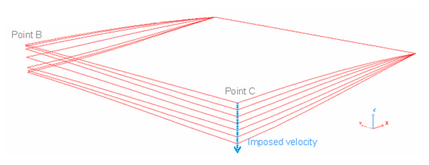
Figure 5. Deformed Configurations during the Snap-thru
Implicit and Explicit Comparison Results
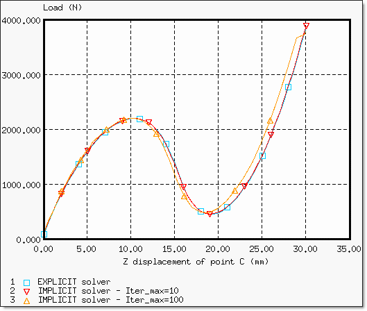
Figure 6. Load Displacement Curve Obtained by Implicit and Explicit Solvers
| Implicit Solver | Explicit Solver | |
|---|---|---|
| Normalized CPU | 1 | 2.45 |
| Cycles (normalized) | 1 | 237 |
In comparison with the implicit computation, which uses a maximum time step of 10 ms, the saved CPU time using a maximum time step fixed at 100 ms, approximately corresponds to factor 4.