Explicit Example
An imposed velocity is applied onto a shallow cylindrical roof at its midpoint. The analysis uses an explicit approach.
The purpose of this example is to study a snap-thru problem with a single instability. Thus, a structure that will bend when under a load is used. The results are compared to the references solution. 1
Options and Keywords Used
Node time histories do not indicate the pressure output. In order to obtain such output at point C, a rigid body must be created at this point. Point C has a constant imposed velocity of -0.01 ms-1in the Z direction. Its displacement is linked proportionally to time.
- Edge BC is fixed in an X translation, and in Y and Z rotations (symmetry conditions).
- Edge CD is fixed in a Y translation, and in X and Z rotations (Idem).
- Edge DA is fixed in X, Y, Z translations, and in X and Z rotations.
- Point C is fixed in X, Y translations, and in X, Y, Z rotations.
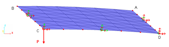
Figure 1. Boundary Conditions
Input Files
- Explicit solvers
- <install_directory>/hwsolvers/demos/radioss/example/02_Snap-through/Explicit_solver/SNAP_EXP*
Model Description
A shallow cylindrical roof, pinned along its straight edges upon which an imposed velocity is applied at its mid-point.
Units: mm, ms, g, N, MPa
- l
- 254 mm
- R
- 2540 mm
- Shell thickness
- t = 12.7 mm
- 0.1 rad
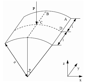
Figure 2. Geometrical Data of the Problem
- Material Properties
- Initial density
- 7.85x10⁻³
- Young's modulus
- 3102.75
- Poisson ratio
- 0.3
Model Method
The structure is considered perfect, having no defects. To take account of the symmetries, only a quarter of the shell is modeled (surface ABCD).
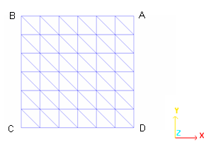
Figure 3. T3 Mesh
- Shell Properties
- Thickness
- 12.7 mm
- BT Elasto-plastic Hourglass formulation
- Ishell= 3
Results
Curves and Animations
Only a quarter of the total load is applied due to the symmetry. Therefore, force Fz of the rigid body, as indicated in the Time History, must be multiplied by 4 in order to obtain force, P.
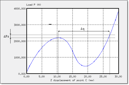
Figure 4. Load P versus Displacement of Point C: Snap-thru Instability
The displacement of point C is indicated in its absolute value. The curve illustrates the characteristic behavior of the instability of a snap-thru. Beyond the limit load, an infinite increase in load will cause a considerable increase in displacement due to the collapsing of the shell.
The first extreme defines the limit load =2208.5 N (displacement of point C = 10.5 mm).
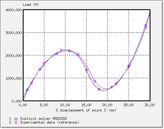
Figure 5. Comparison between a Reference Curve and a Curve Obtained Using Radioss
The difference between the two curves is approximately 10% for reduced displacements (up to 5 mm) and slightly more (15%) for the higher nonlinear part of the curve (between 5 and 20 mm). For displacements exceeding 20 mm, the curves are shown much closer together.
| Deformed Mesh (profile view) - Displacement Norm |
|---|
 Initial configuration |
 Start of snap-thru |
 Large motion phase |
 Stable configuration |
 Loading with a new structural rigidity |