RD-E: 0903 Interfaces Study
Comparison of results obtained using different interfaces.
Options and Keywords Used
- The relaxation value by default, equal to 1
- The period to be damped (less than or equal to the largest period of the system)
- without relaxation
- with relaxation
with
- Inputs
- = 1
- = 0.2
The dynamic problem (impact between balls) is considered in a second run managed by the second Engine file (*_0002.rad) with a time running from 30 ms to 130 ms.
Input Files
- Inter_7_Penalty
- <install_directory>/hwsolvers/demos/radioss/example/09_Billiards/Contact_modelling/Inter_7_Penalty/TEST7P*
- Inter_7_Lagrangian
- <install_directory>/hwsolvers/demos/radioss/example/09_Billiards/Contact_modelling/Inter_7_Lagrangian/TEST7L*
- Inter_16_tied
- <install_directory>/hwsolvers/demos/radioss/example/09_Billiards/Contact_modelling/Inter_16_tied/TEST16T*
- Inter_16_sliding
- <install_directory>/hwsolvers/demos/radioss/example/09_Billiards/Contact_modelling/Inter_16_sliding/TEST16S*
- Inter_17_tied
- <install_directory>/hwsolvers/demos/radioss/example/09_Billiards/Contact_modelling/Inter_17_tied/TEST17ST*
- Inter_17_sliding
- <install_directory>/hwsolvers/demos/radioss/example/09_Billiards/Contact_modelling/Inter_17_sliding/TEST17S*
Model Description
The balls and the table have the same properties as previously defined. The dimensions of the table are 900 mm x 450 mm x 25 mm and the balls' diameter is 50.8 mm.
- Interfaces Used in the Problems
- TYPE16 (Lagrange Multipliers) tied or sliding
- Secondary nodes/main solids contact
- TYPE17 (Lagrange Multipliers) tied or sliding
- Secondary 16-node shells/main 16-node shells contact
- TYPE7 (Lagrange Multipliers)
- Secondary nodes/main surface contact
- TYPE7 (Penalty) sliding
- Secondary nodes/main surface contact
Model Method
The TYPE16 interface defines contact between a group of nodes (secondary) and a curved surface of quadratic elements (main part). The TYPE17 interface is used for modeling a surface-to-surface contact. For both interfaces, the Lagrange Multipliers method is used to apply the contact conditions; gaps are not required. Contact between the balls and the table is set as tied or sliding. Contact between the balls themselves is always considered as sliding. The TYPE7 interface enables the simulation of the most general contact types occurring between a main surface and a set of secondary nodes. The Coulomb friction between surfaces is not modeled here (sliding contact) and the gap is fixed at 0.1 mm. The other parameters are set to default values.
The TYPE7 interface with the Penalty method is not available with 16-node thick shell elements. Thus, brick elements replace the 16-nodes shells in this case (check in the input file).
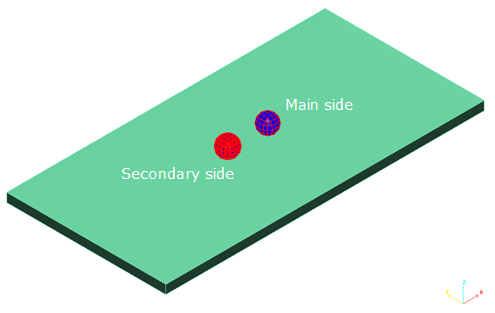
Figure 1. Definition of Secondary and Main Sides for Contact
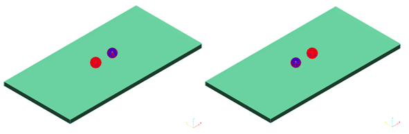
Figure 2. Symmetrical Configuration of the TYPE7 Interface using the Penalty Method
- Interface
- Secondary (red) and Main (blue) Objects
- TYPE16 - tied
- Secondary: nodes
- TYPE16 - sliding
- Secondary: nodes
- TYPE17 - tied
- Secondary: 16-node shell
- TYPE17 - sliding
- Secondary: 16-node shell
- TYPE7 - Lagrange Multipliers
- Secondary: nodes
- TYPE7 - Penalty method
- Secondary: nodes
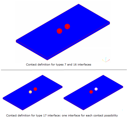
Figure 3. Definition of Secondary and Main Objects for Balls/Table Contacts
- Interface
- Secondary (red) and Main (blue) Objects
- TYPE16 - tied
- Secondary: nodes
- TYPE16 - sliding
- Secondary: nodes
- TYPE17 - tied
- Secondary: 16-node shell
- TYPE17 - sliding
- Secondary: 16-node shell
- TYPE7 - Lagrange Multipliers
- Secondary: nodes
- TYPE7 - Penalty method
- Secondary: nodes
Pre-loading: quasi-static gravity loading to reach static equilibrium.
The explicit time integration scheme starts with nodal acceleration computation. It is efficient for the simulation of dynamic loadings. However, a quasi-static simulation via a dynamic resolution method needs to minimize the dynamic effects for converging towards static equilibrium and describes the pre-loading case before the dynamic analysis. Thus, the quasi-static solution of gravity loading on the model shows a steady state in the transient response.
Results
Kinetic Energy Transmission between Balls during Collision

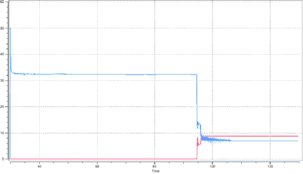 Figure 4. TYPE17 Interface. Contact between quadratic surfaces Balls/table contact: tied / Ball/ball
contact: sliding
Figure 4. TYPE17 Interface. Contact between quadratic surfaces Balls/table contact: tied / Ball/ball
contact: sliding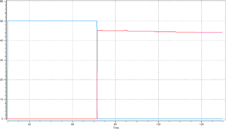 Figure 5. TYPE17 Interface. Contact between quadratic surfaces Balls/table contact: sliding /
Ball/ball contact: sliding
Figure 5. TYPE17 Interface. Contact between quadratic surfaces Balls/table contact: sliding /
Ball/ball contact: sliding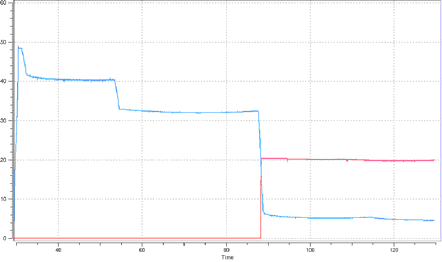
Figure 6. TYPE16 Interface. Contact nodes/quadratic surface Balls/table contact: tied / Ball/ball contact: sliding
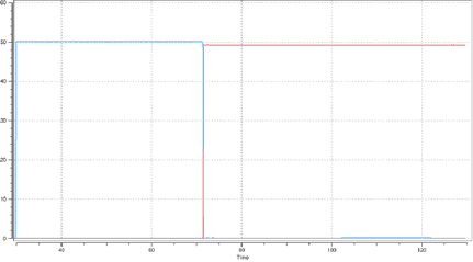 Figure 7. TYPE16 Interface. Contact nodes/quadratic surface Balls/table contact: sliding / Ball/ball
contact: sliding
Figure 7. TYPE16 Interface. Contact nodes/quadratic surface Balls/table contact: sliding / Ball/ball
contact: sliding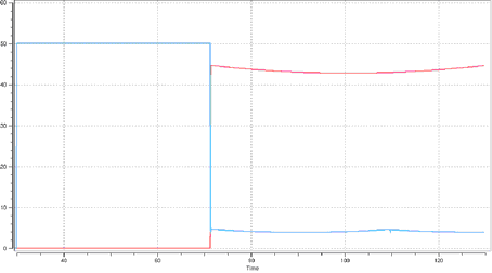 Figure 8. TYPE7 Interface: Lagrange Multipliers Method. Contact nodes/linear surface (sliding contact)
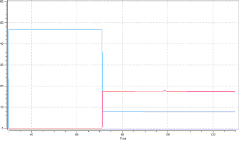 Figure 9. TYPE7 Interface: Penalty Method. Contact nodes/linear surface Balls/table contact: sliding / Ball/ball
contact: sliding
Figure 9. TYPE7 Interface: Penalty Method. Contact nodes/linear surface Balls/table contact: sliding / Ball/ball
contact: slidingConclusion
| Interface 16 Tied | Interface 16 Sliding | Interface
17 Tied |
Interface 17 Sliding | Interface
7 Lagrange Multipliers |
Interface
7 Penalty |
|
|---|---|---|---|---|---|---|
| Cycles | 241392 | 241385 | 241387 | 241385 | 241385 | 773099 |
| Error on Energy | -30.8% | -1.4% | -55.5% | -10.8% | -1.2% | -46.1% |
| Rolling | yes | no | yes | no | no | no |
| Momentum Transmission | partial | quasi-perfect | partial | good | good | partial |
| Quadratic surface | main side | main side | main and secondary sides | main and secondary sides | no | no |
A non-elastic collision appears using the TYPE7 interface Penalty method. After impact, each ball has about half of the initial velocity. The momentum transmission is partial and can be improved by increasing the stiffness of the interface despite the hourglass energy and degradation of the energy assessment.
Error on energy is more noticeable for interfaces using the Tied option, due to taking into account the rolling simulation.
This study shows the high sensitivity of the numerical algorithms for the modeling impact on elastic balls. Regarding the interface type, the kinematics of the problem and the transmission of momentum are more or less satisfactory. TYPE16 interface allows good results to be obtained.