Incompressible Tube Element
Incompressible Tube Element Description and Quick Guide
The three elements shown here: Incompressible Tube, Elastic Pipe, and Inelastic Pipe, fall under the category of Incompressible Tubes. These elements solve the 1D Navier-Stokes equations with the option to incorporate friction, heat transfer, area change, rotation, buoyancy, and bend geometry effects.
The Incompressible Tube is the generic, all-purpose tube for incompressible models.
The Elastic Pipe includes the transient pressure wave effects also known as Water Hammer.
The Inelastic Pipe allows the user to pick from a built-in set of piping size and has a somewhat simplified set of inputs from the Incompressible Tube.
All three types of Incompressible Tubes must be used with fluids in the liquid phase.
The incompressible tube is subdivided into axial segments that can have unique inputs for geometry, heat transfer, and friction. The incompressible tube can also be subdivided into circumferential segments that can have unique heat transfer and friction.
Each segment of an incompressible tube can be associated with a thermal network node and convector.
Incompressible Tube Element Inputs
Table of the inputs for the incompressible tube element.
| Element Specific Input Variables | |||||||||||||||||||||||||||||||||||||||||||||||
| Index | UI Name (.flo label) | Description | |||||||||||||||||||||||||||||||||||||||||||||
| 1 | Cross-Sectional Shape (CS_SHAPE) |
Specifies method for defining tube geometry parameters: hydraulic diameter (DHI), wetted perimeter (PWI), and flow area (AFI). The cross-section shape is also used to find an effective hydraulic diameter. The following typical settings are set automatically by the GUI based on the selections made for Geometric Input Type and Size. 1: Circular tube with uniform area along the length of the tube. A single value for area is set in STATION_CS_AREAS 2: Circular tube with uniform diameter along the length of the tube. A single value for diameter is set in STATION_HYDDIAMS_OR_PERIMS 6: Arbitrary cross-sectional shape with uniform area and hydraulic diameter along the length of the tube. A single value for area is set on STATION_CS_AREAS and a single value for hydraulic diameter is set on STATION_HYDDIAMS_OR_PERIMS 7: Arbitrary cross-sectional shape with uniform area and wetted perimeter along the length of the tube. A single value for area is set on STATION_CS_AREAS and a single value for wetted perimeter is set on STATION_HYDDIAMS_OR_PERIMS 11: Tapered circular tube with area specified at inlet and exit. Assumes linear tapering of area. Inlet and exit area values are set on STATION_CS_AREAS 12: Tapered circular tube with diameter specified at inlet and exit. Assumes linear tapering of diameter. Inlet and exit diameter values are set on STATION_HYDDIAMS_OR_PERIMS 16: Tapered arbitrary cross-section shaped tube with area and hydraulic diameter specified at inlet and exit. Assumes linear tapering of area and hydraulic diameter. Inlet and exit area values are set on STATION_CS_AREAS. Inlet and exit hydraulic diameter values are set on STATION_HYDDIAMS_OR_PERIMS. 17: Tapered arbitrary cross-section shaped tube with area and wetted perimeter specified at inlet and exit. Assumes linear tapering of area and wetted perimeter. Inlet and exit area values are set on STATION_CS_AREAS. Inlet and exit wetted perimeter values are set on STATION_HYDDIAMS_OR_PERIMS. 21: Circular tube with area specified each station. Assumes linear tapering of area between stations. NUM_STATIONS number of area values are set on STATION_CS_AREAS 22: Circular tube with diameter specified each station. Assumes linear tapering of diameter between stations. NUM_STATIONS number of diameter values are set on STATION_HYDDIAMS_OR_PERIMS 26: Arbitrary cross-section shaped tube with area and hydraulic diameter specified each station. Assumes linear tapering of area and hydraulic diameter between stations. NUM_STATIONS number of area values are set on STATION_CS_AREAS. NUM_STATIONS number of hydraulic diameter values are set on STATION_HYDDIAMS_OR_PERIMS 27: Arbitrary cross-section shaped tube with area and wetted perimeter specified each station. Assumes linear tapering of area and wetted perimeter between stations. NUM_STATIONS number of area values are set on. There are additional setting for triangle, rectangle, elliptical and annular shapes. |
|||||||||||||||||||||||||||||||||||||||||||||
| 2 | Number of Stations (NUM_STATIONS) |
Number of stations in the tube. Station 1 is at the inlet plane; station NUM_STATIONS is at the exit plane. NSTA can range from 2 to unlimited. During the solution process, the tube will be discretized into NUM_STATIONS minus one segments with average temperatures, pressures, and Reynolds Numbers for each segment. A tube should be modelled with at least five stations. The number of stations can have a big impact on the convergence of attached chambers. If a chamber attached to this element is having difficulty converging, try increasing the number of stations. Of course, analysis speed may decrease as the number of stations increase. |
|||||||||||||||||||||||||||||||||||||||||||||
| 3 | Number of tube wall sides (NUM_WALL_SIDES) |
|
|||||||||||||||||||||||||||||||||||||||||||||
| 4 | Number of bends (NUM_BENDS) | Number of bends in the tube. Each bend is defined by a bend radius, bend angle, location in the tube (either distance from start of tube, or a specified straight segment length between bends), loss multiplier and combination angle. | |||||||||||||||||||||||||||||||||||||||||||||
| 5 |
Tube Length (LENGTH) |
Length of the tube in inches. Do not include length within bends unless the bend losses are not otherwise accounted. | |||||||||||||||||||||||||||||||||||||||||||||
| 6 | STATION_MODE |
Flag specifying station location definitions. 0: Stations are uniformly distributed along the length of the tube 1: Station location is defined as a percentage of length of the tube. User specifies percentage for each station in the STATION_LOCATIONS array. Valid values are 0-100. 2: Station location is defined as distance from the start of the tube. User specifies distance from start for each station in the STATION_LOCATIONS array. Valid values are 0-LENGTH |
|||||||||||||||||||||||||||||||||||||||||||||
| 7 | Turbulent Friction Relation (FRIC_RELATION) |
A flag that specifies which friction relation is used. 0.0: Smooth Wall Power law (Abuaf) 1.0: Swamee-Jain (approx. to Colebrook-White) Swamee-Jain (1.0) is recommended for non-zero roughness. |
|||||||||||||||||||||||||||||||||||||||||||||
| 8 |
Roughness type (ROUGH_TYPE) |
Flag specifying measurement method of user-input ROUGHNESS value. Roughness values will be converted to san-grain roughness equivalent. For more information see Friction Correlations section in General Functions and Routines. 0: Equivalent sand-grain roughness 1: Average absolute roughness 2: Root mean square roughness 3: Peak-to-valley roughness |
|||||||||||||||||||||||||||||||||||||||||||||
| 9 |
HTC Relation (HTC_RELATION) |
The “Duct Flow” Nu correlation used for turbulent flow. See the “HTC Correlations” in the “General Functions and Routines” section for the equations. -2) User Input Nu -1) User Input HTC 1) Lapides-Goldstein 2) Dittus-Boelter 3) Sieder-Tate Combo 4) Gnielinski Combo 5) Bhatti-Shah 7) Sieder-Tate Turbulent Only 8) Gnielinski-Turbulent Only |
|||||||||||||||||||||||||||||||||||||||||||||
| 10 |
Heat Transfer Inlet Effects Flag (HT_INLET_EFF) |
Flag specifying heat transfer inlet effects applied for the tube. See the Heat Transfer Coefficients (HTC) section in General Functions and Routines. 0: No inlet effects 1: Abrupt local or uniform average inlet effects 3: Abrupt average inlet effects 4: Uniform local inlet effects 5: Between uniform average and local inlet effects 6: Between abrupt average and local inlet effects |
|||||||||||||||||||||||||||||||||||||||||||||
| 11 | Portion of Ustrm Cham. Dyn. Head Lost (DQ_IN) |
Inlet dynamic head loss. Valid range is 0.0 to 1.0 inclusive. An entry outside this range will cause a warning message and the value used will be 0 or 1 (whichever value is closest to the entry). If DQ_IN > 0 and the upstream chamber has a positive component of relative velocity aligned with the centerline of the orifice, the driving pressure will be reduced by the equation:
(Default value = 0.) |
|||||||||||||||||||||||||||||||||||||||||||||
| 12 | Rotor Index (RPMSEL) |
Element rotational speed pointer. 0.0: Specifies a stationary element. 1.0: Rotor 1, RPM = general data ELERPM(1). 2.0: Rotor 2, RPM = general data ELERPM(2). 3.0: Rotor 3, RPM = general data ELERPM(3). |
|||||||||||||||||||||||||||||||||||||||||||||
| 13 |
Gravity Multiplier (GRAV_MULT) |
Multiplier on the constant for acceleration due to gravity, Gc. Gc is nominally equal to 32.17405 lbm-ft/lbt-sec2. | |||||||||||||||||||||||||||||||||||||||||||||
| 14 |
Element Inlet Orientation: Tangential Angle (THETA) |
Angle (deg) between the element centerline at the entrance of the element and the reference direction. If the element is rotating or directly connected to one or more rotating elements, the reference direction is defined as parallel to the engine centerline and the angle is the projected angle in the tangential direction. Otherwise, the reference direction is arbitrary but assumed to be the same as the reference direction for all other elements attached to the upstream chamber. Theta for an element downstream of a plenum chamber has no impact on the solution except to set the default value of THETA_EX. (See also THETA_EX) |
|||||||||||||||||||||||||||||||||||||||||||||
| 15 |
Element Inlet Orientation: Radial Angle (PHI) |
Angle (deg) between the element centerline at the entrance of the element and the THETA direction. (spherical coordinate system) Phi for an element downstream of a plenum chamber has no impact on the solution except to set the default value of PHI_EX. (See also PHI_EX) |
|||||||||||||||||||||||||||||||||||||||||||||
|
16 17 18 |
Exit K Loss: Axial (K_EXIT_Z) Tangential (K_EXIT_U) Radial (K_EXIT_R) |
Head loss factors in the Z, U, and R directions based on the spherical coordinate system of theta and phi. Z = the axial direction. (theta=0 and phi=0) U = the tangential direction. (theta=90 and phi=0) R = the radial direction. (theta=0 and phi=90) Valid values of K_EXIT_i (i = Z, U, R) range from zero (default) to one. The three loss factors reduce the corresponding three components of velocity exiting the element.
(Default value provides no loss, K_EXIT_i=0) |
|||||||||||||||||||||||||||||||||||||||||||||
| 19 | Element Exit Orientation: Tangential Angle (THETA_EX) |
Angle (deg) between the element exit centerline and the reference direction. THETA_EX is an optional variable to be used if the orientation of the element exit differs from that of the element inlet. The default value (THETA_EX = -999) will result in the assumption that THETA_EX = THETA. Other values will be interpreted in the manner presented in the description of THETA. |
|||||||||||||||||||||||||||||||||||||||||||||
| 20 | Element Exit Orientation: Radial Angle (PHI_EX) |
Angle (deg) between the element exit centerline and the THETA_EX direction. PHI_EX is an optional variable to be used if the orientation of the element exit differs from that of the element inlet. The default value (PHI_EX = -999) will result in the assumption that PHI_EX = PHI. Other values will be interpreted in the manner presented in the description of PHI. |
|||||||||||||||||||||||||||||||||||||||||||||
| 21 |
Nusselt Number for Laminar Flow (NU_LAM) |
Nusselt number used in the laminar flow region (defaults to 4.36) | |||||||||||||||||||||||||||||||||||||||||||||
| 22 |
Elastic Pipe or (Incompressible Tube and Inelastic Pipe) (ELASTIC_FLAG) |
0 = No transient water hammer calculations for Incompressible Tube and Inelastic Pipe 1 = transient water hammer calculations for Elastic Pipe |
|||||||||||||||||||||||||||||||||||||||||||||
| 23 |
Wall Thickness (WALL_THICKNESS) |
Pipe wall thickness for elastic pipe (water hammer) calculations | |||||||||||||||||||||||||||||||||||||||||||||
| 24 |
Exit Static Pressure Tolerance Value (PRESSURE_TOL) |
User defined exit static pressure convergence tolerance. Caution should be used when increasing this very much above the default value. Defaults to 0.000001 psia. |
|||||||||||||||||||||||||||||||||||||||||||||
| 25 |
Number of Axial Grid Cells (NSTA_ELASTIC) |
Number of cells along the length of the tube for elastic pipe (water hammer) calculations. Should be greater than (5 times as many) the number of tube stations. | |||||||||||||||||||||||||||||||||||||||||||||
| 26 |
Aspect Ratio (ASPECT_RATIO) |
The aspect ratio of the tube cross section for an Arbitrary-Shape cross section. The aspect ratio should be between 0 and 1. | |||||||||||||||||||||||||||||||||||||||||||||
| 27 |
Laminar Friction Effects (LAMR_FRIC_RLTN) |
Laminar friction effects to use at the duct inlet. See the “Friction Correlations” in the “General Functions and Routines” section for the equations.
0) Off, assume fully developed laminar flow. 1) Muzychka-Yovanovich |
|||||||||||||||||||||||||||||||||||||||||||||
| 28 |
Laminar HTC Relation (NU_LAM_METHOD) |
The “Duct Flow” Nu correlation used for laminar flow. See the “HTC Correlations” in the “General Functions and Routines” section for the equations. 0) User Input Nu 1,4,5) Muzychka-Yovanovich 2) Hausen |
|||||||||||||||||||||||||||||||||||||||||||||
| 29 |
NONE (PROPS_METHOD) |
No applicable | |||||||||||||||||||||||||||||||||||||||||||||
| 30 |
Poisson Ratio (POISSON_RATIO) |
Tube wall material property for elastic pipe (water hammer) calculations. | |||||||||||||||||||||||||||||||||||||||||||||
| 32 |
Inlet Head Loss Type (K_IN_METHOD) |
The type of inlet losses. K – Incompr Loss Coef Kin = inlet head loss / dynamic head, or
Cd – Compr Loss Coef Upstream Cross Flow
The tube inlet loss is assumed to be due to a cross flow velocity at the tube’s inlet and is calculated according to Ref. 6. The data used is for a tube with L/D > 2.83, where the flow has recovered from the inlet effects and is at right angles to the cross flow. The method is valid for both upstream momentum and upstream inertial chambers. It is not valid for upstream plenum chambers. |
|||||||||||||||||||||||||||||||||||||||||||||
| 31,33-35 | (FUTURE) | Reserved for future development | |||||||||||||||||||||||||||||||||||||||||||||
| 36 |
Bend Input Mode (BEND_INPUT_MODE) |
Flag indicating how the locations of bends are defined.
0: Bend location is distance from start of the tube in inches.
1: Bend location is defined by the distance of straight tube length between the end of the previous bend (or inlet, if it is the first bend) and the beginning of the current bend |
|||||||||||||||||||||||||||||||||||||||||||||
| 37 |
Laminar-to-Transition Reynolds Number (RE_LAM) |
Reynolds number below which flow is assumed to be laminar | |||||||||||||||||||||||||||||||||||||||||||||
| 38 |
Transition-to-Turbulent Reynolds Number (RE_TURB) |
Reynolds number above which flow is assumed to be turbulent. Flow at Reynolds numbers between RE_LAM and RE_TURB are assumed to be in the transition region. | |||||||||||||||||||||||||||||||||||||||||||||
| 39 |
Friction Type (FRIC_TYPE) |
Friction factor output type. 1: Darcy friction factor 2: Fanning friction factor |
|||||||||||||||||||||||||||||||||||||||||||||
| 40 |
Starting Length (STLEN) |
Starting length (in) used for the HTC inlet multiplier. Used to modify X in calculating hx/ho:
where Xmeas = Distance from tube inlet (station 1). At station 1, X equals STLEN. If one physical tube is modelled as two or more elements strung together, STLEN should include the cumulative length of all tube elements leading into the current element unless something physical re-establishes the boundary layer. |
|||||||||||||||||||||||||||||||||||||||||||||
| 41 |
Inlet Head Loss (K_INLET) |
Inlet head loss. This is either a K or Cd depending on K_IN_METHOD. |
|||||||||||||||||||||||||||||||||||||||||||||
| 42 |
Bulk Modulus (BULK_MOD) |
Fluid material property for elastic pipe (water hammer) calculations. | |||||||||||||||||||||||||||||||||||||||||||||
| 43 |
Water Hammer Inputs (WALL_MATERIAL) |
Either option for wave speed estimate or a material identifier for elastic pipe (water hammer) calculations. 0 = User inputs wave speed 1 = User inputs Young’s modulus |
|||||||||||||||||||||||||||||||||||||||||||||
| 44 |
Young’s Modulus (YOUNGS_MOD) |
Tube wall material property for elastic pipe (water hammer) calculations. | |||||||||||||||||||||||||||||||||||||||||||||
| 45 |
Wave Velocity (WAVE_SPEED) |
Wave speed estimate for elastic pipe (water hammer) calculations. | |||||||||||||||||||||||||||||||||||||||||||||
| A1 |
Bend Radius (BEND_RADIUS) (array of 20 values in 4 lines of 5 each, NUM_BENDS values used) |
Radius (in) of bend along tube centerline. (See ‘ r ’ from graphic for COMBINATION_ANGLE below) Each bend counted in NUM_BENDS must have a specified bend radius. Enter bends in order based on distance from beginning of tube (DIST_FR_STRT). |
|||||||||||||||||||||||||||||||||||||||||||||
| A2 |
Bend Angle (BEND_ANGLE) (array of 20 values in 4 lines of 5 each, NUM_BENDS values used) |
Angle (deg) between the entering and exiting lengths of the bend. Each bend must have a specified angle. The maximum bend angle is 180°. |
|||||||||||||||||||||||||||||||||||||||||||||
| A3 |
Distance from Start (DISTANCE) (array of 20 values in 4 lines of 5 each, NUM_BENDS values used) |
Array of values that indicate bend location in the tube. The interpretation of the values in the array depends on the value of BEND_INPUT_MODE: BEND_INPUT_MODE = 0: DISTANCE is cumulative straight tube segment length (in.) to the start of the current bend, BEND_INPUT_MODE = 1: DISTANCE is straight segment length (in.) from end of the previous bend (or inlet if it is the first bend in the tube) to the start of the current bend. |
|||||||||||||||||||||||||||||||||||||||||||||
| A4 |
Loss Multiplier (LOSS_MULT) (array of 20 values in 4 lines of 5 each, NUM_BENDS values used) |
Loss multiplier for each bend (Default = 1.0). | |||||||||||||||||||||||||||||||||||||||||||||
| A5 |
Combination Angle (COMBINATION_ANGLE) (array of 20 values in 4 lines of 5 each, NUM_BENDS minus one values used) |
Relative angle (deg) between two bends in series. The number of COMBINATION_ANGLE entries will be NUM_BENDS – 1. The first entry will be the combination angle between bends 1 and 2. A COMBINATION_ANGLE of 0 degrees defines an ‘S’ shaped bend and 180 degrees defines a ‘U’ shaped bend. The allowable range is 0 to 180 degrees. 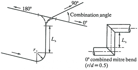 |
|||||||||||||||||||||||||||||||||||||||||||||
| A6 |
STATION_LOCATIONS (Dynamic array of NUM_STATIONS values) |
Dynamic array of NUM_STATIONS station locations, specified as a percentage of length, a fraction of length, or a distance from start of tube, depending on the value of STATION_MODE. For STATION_MODE = 0 (uniformly distributed), this array will not be used. | |||||||||||||||||||||||||||||||||||||||||||||
| A7 |
STATION_RADII (Dynamic array of NUM_STATIONS values) |
Dynamic array of NUM_STATIONS station radii in inches. Only applicable for rotating tubes, i.e. RPMSEL not equal to 0. | |||||||||||||||||||||||||||||||||||||||||||||
| A8 |
STATION_HEIGHTS (Dynamic array of NUM_STATIONS values) |
Dynamic array of NUM_STATIONS station heights in inches. Only applicable for stationary tubes, i.e. RPMSEL = 0, and when gravitational effects are enabled. Station height is defined as distance above a datum and is used to determine gravitational effects on the fluid. | |||||||||||||||||||||||||||||||||||||||||||||
| A9 |
Station cross-section areas (STATION_CS_AREAS, dynamic array, length depends on value of CS_SHAPE) |
Dynamic array of station cross-section areas. Length of the array is determined by the value of CS_SHAPE. STATION_CS_AREAS is only used for CS_SHAPE = 1, 6, 7, 11, 16, 17, 21, 26, or 27
|
|||||||||||||||||||||||||||||||||||||||||||||
| A10 |
Station hydraulic diameter or wetted perimeter (STATION_HYDDIAMS_OR_PERIMS, dynamic array, length and meaning of value depends on value of CS_SHAPE) |
Dynamic array of station hydraulic diameter or perimeter. Length of and meaning of value in the array is determined by the value of CS_SHAPE. STATION_HYDDIAMS_OR_PERIMS is only used for CS_SHAPE = 2, 6, 7, 12, 16, 17, 22, 26, or 27
|
|||||||||||||||||||||||||||||||||||||||||||||
| A11 |
WALL_SIDE_FRACTIONS (Dynamic array of length NUM_WALL_SIDES) |
Array of length NUM_WALL_SIDES specifying the portion of the tube perimeter represented by each wall side (segment). WALL_SIDE_FRACTIONS can be input as either a fraction or a percentage. If input as a fraction:
And if input as a percentage:
Wall sides cover the length of the tube and thus apply at every station. |
|||||||||||||||||||||||||||||||||||||||||||||
| A12 |
WALL_SIDE_TYPES (Dynamic array of length NUM_WALL_SIDES) |
Array of length NUM_WALL_SIDES specifying the surface type of each wall side (segment). 0: Smooth surface 1: Rough surface 2: Turbulated surface For types 1 and 2, additional inputs are required to define roughness and/or turbulator geometry. Wall sides cover the length of the tube and thus apply at every station. |
|||||||||||||||||||||||||||||||||||||||||||||
| A13 |
LOSS_MODE_ON_EACH_SIDE (Dynamic array of length NUM_WALL_SIDES) |
Array of length NUM_WALL_SIDES specifying the momentum loss calculation method for each wall side (segment). 0: No momentum loss 1: Specified roughness, uniform along tube length 2: Specified friction coefficient, uniform along tube length 3: Specified Kloss, uniform along tube length 4: Specified friction multiplier applied to calculated friction, uniform along tube length 12: Linearly tapered friction coefficient, specified at inlet and exit 14: Linearly tapered friction multiplier applied to calculated friction, specified at inlet and exit 21: Specified roughness for each tube segment (between stations) 22: Specified friction coefficient for each tube segment (between stations) 23: Specified Kloss for each tube segment (between stations) 24: Specified friction multiplier applied to calculated friction for each tube segment (between stations) The choice of LOSS_MODE_ON_EACH_SIDE will determine the length of and interpretation of the values in the LOSS_QUANTITIES_ON_SIDE_X arrays Wall sides cover the length of the tube and thus apply at every station. |
|||||||||||||||||||||||||||||||||||||||||||||
| A14 |
HEAT_MODE_ON_EACH_SIDE (Dynamic array of length NUM_WALL_SIDES) |
Array of length NUM_WALL_SIDES specifying the heat transfer calculation method for each wall side (segment). 0: Adiabatic 1: Uniform heat load (Btu/s) 2: Uniform heat load (Btu/lbm) 3: Uniformly distributed delta T (Not implemented) 4: Fixed fluid total temperature at tube exit (Not implemented) 5: Calculated inner wall convection 6: Inner wall convection with constant Nusselt number 7: Inner wall convection with constant heat transfer coefficient 8: Calculated inner wall convection with constant Hmult 16: Inner wall convection with linearly tapered Nusselt number, specified at inlet and exit. 17: Inner wall convection with linearly tapered HTC, specified at inlet and exit. 18: Calculated inner wall convection with linearly tapered Hmult, specified at inlet and exit. 21: Specified heat load (Btu/s) at each tube segment (between stations) 22: Specified heat load (Btu/lbm) at each tube segment (between stations) 23: Specified delta T across each tube segment (between stations) (Not implemented) 24: Specified total temperature at each tube station (Not implemented) 26: Inner wall convection with Nusselt number specified for each tube segment (between stations) 27: Inner wall convection with HTC specified for each tube segment (between stations) 28: Calculated inner wall convection with Hmult specified for each tube segment (between stations) The choice of HEAT_MODE_ON_EACH_SIDE will determine the length of and interpretation of the values in the HEAT_QUANTITIES_ON_SIDE_X arrays Wall sides cover the length of the tube and thus apply at every station. |
|||||||||||||||||||||||||||||||||||||||||||||
| A15 | LOSS_QUANTITIES_ON_SIDE_X |
These arrays hold the loss quantities on side number X. There will be NUM_SIDES number of these arrays in the database and their length and interpretation of contained values is determined by the value of LOSS_MODE_ON_EACH_SIDE as follows:
Note: Interpretation of roughness values
specified for LOSS_QUANTITIES_ON_SIDE_X will depend on the
value of the ROUGH_TYPE input parameter.
|
|||||||||||||||||||||||||||||||||||||||||||||
| A15 | HEAT_QUANTITIES_ON_SIDE_X |
These arrays hold the heat transfer quantities on side number X. There will be NUM_SIDES number of these arrays in the database and their length and interpretation of contained values is determined by the value of LOSS_MODE_ON_EACH_SIDE as follows:
|
|||||||||||||||||||||||||||||||||||||||||||||
| A15 |
HEAT_QUANTITIES_ON_SIDE_X (Continued) |
Note: For Heat Modes using calculated
inner wall convection, the method of heat transfer
calculation is determined by the value of the HTC_RELATION
input parameter.
|
|||||||||||||||||||||||||||||||||||||||||||||
| A16 |
WALL_TEMPERATURE_ON_SIDE_X (Dynamic array, number of values is input by the user) |
Surface temperature of the tube wall for use in heat transfer and fluid calculations. The user has three options for number of values to input for wall temperature. The size of the array determines how the values in the array are determined:
|
|||||||||||||||||||||||||||||||||||||||||||||
Incompressible Tube Element Theory Manual
The incompressible tube element routine simulates incompressible liquid or gas flow through a passage where friction is a significant pressure loss mechanism. Both laminar and turbulent flows are accommodated by the routine as is heat transfer with either internal turbulators or with conduction/convection/radiation using thermal networks.
The body of the tube is divided into segments of arbitrary length, the number of segments, typically (but not limited to) between 5 and 15, being that specified in the input file. The beginning and end of each segment is represented as a “station” so there is one more station than the number of segments used for the tube. The geometry of the tube flow passage is defined by a combination of two of the three input variables, flow area, hydraulic diameter, and wetted perimeter, specified for each of the tube stations, the remaining variable being calculated using the equation:
The tube routine is divided into two main sections: a flow direction calculation and a flow iteration loop. In the flow direction section, the procedures described in the paragraphs on computing the element flow inlet and outlet conditions are employed to define the inlet driving pressure (PTS), the inlet temperature, the secondary fluid mass fraction, and the exit back pressure (PSEB). If the tube is rotating and its inlet and outlet are at different radii, an estimate of the pumping effect due to rotation is used to compute an effective inlet pressure, PTSM. The procedure used to calculate the pressure ratio, PTSM / PTS, is identical to that for a forced vortex turning at the specified element RPM. If PTS (or PTSM) is greater than PSEB, these pressures are employed with a simple overall flow coefficient, based on inlet pressure drop and estimated friction effect, to estimate the fluid velocity at the tube exit plane. If PTS (or PTSM) is less than PSEB, the calculation is repeated with the flow direction reversed.
The mass, momentum, and energy conservation must be maintained along the length of the tube. The methods used are described here.
Mass Equation
The continuity equation is given as:
Momentum Equation
The momentum equation for an incompressible tube can be written as (Bernoulli’s equation) [Ref 3]:

The kinetic energy term can be re-written as:
And the momentum equation can be re-written as:

The kinetic energy term can be broken down further as:
This decomposition will be used because for incompressible liquids, the density changes will not be large, but there might be significant velocity changes along the tube.
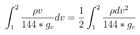
The momentum equation with this implemented is:

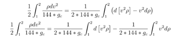
The left-hand side of the equation above can be integrated analytically, while the right-hand side must be integrated numerically:

Note that:
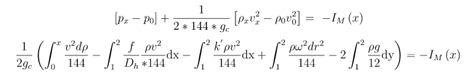
Also, define total pressure as:
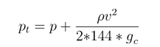
To obtain:
Note that this Is the first order Taylor expansion of compressible relation in the incompressible limit.
can be calculated using the trapezoidal rule as shown below:

Flow Function
Continuity at the tube exit plane is defined by:
Where:
Consider, as defined in the Momentum Equation section:
And:
which yields:
We can rearrange this equation to obtain the flow function as:
Inlet and Exit Plane Calculations
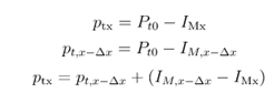
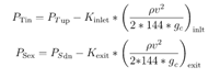
There might be pressure losses at the inlet and exit planes of the incompressible tube element due to bends and junctions. In such cases, the loss coefficients and the pressure terms become:
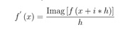
Flow Derivatives
The Flow Simulator solver uses Newton-Raphson method to find a solution and requires the flow rate derivatives and . The calculation method is based on a Taylor series expansion of a complex valued function:

Take the imaginary part of the equation above to obtain:
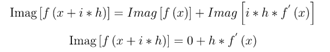
The first-order derivative of the above equation becomes:
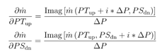
Similarly, the first order flow derivatives required by the Flow Simulator solver are given as:
Energy Equation
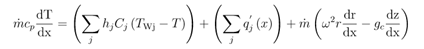
Start with the differential form of the steady state energy balance equation:
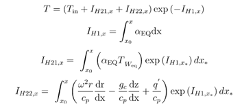
The incompressible tube uses the following energy integral [ref 5 section 1.6]:
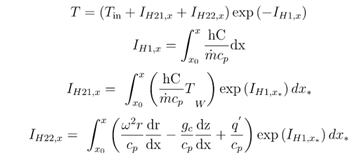
These integrals are calculated in a semi-analytic way.
Integral is calculated as:
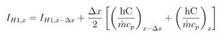
Integral is calculated as:

Where:
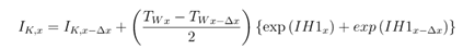
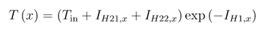
Integral is calculated as:

Finally, temperature at location x is calculated as:
Multiple Wall Segment Case
In the case of an incompressible tube with multiple wall segments defined around the circumference of the tube, the differential form of the energy balance equation becomes:
where j is an individual circumferential wall segment.
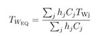
Taking the first term on the right-hand side of the above equation:
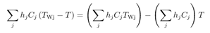
In this equation, only the coefficients are different, and we can calculate an equivalent wall temperature:
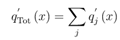
Similarly, the total amount of external heat can be obtained:
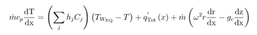
And the differential form of the energy balance equation becomes:
In this case, the following integrals must be used to calculate temperature:
where:

Coupling with the Thermal Network Solver
The total amount of heat added to the fluid is given by:
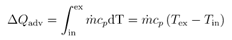
Heat added, , is a result of convection from the tube wall:
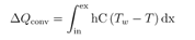
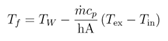
Wall temperature along a segment is constant and we assume that there is a fluid temperature that satisfies:
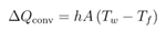
The fluid temperature can be calculated as:
Incompressible Tube Element Outputs
The following listing provides details about the elements output variables.
| Name | Description | Units |
|---|---|---|
| CROSS-SECTION: | Shape of tube cross-section | (None) |
| LENGTH: | Length of the tube | Inch, m |
| NUM_STATIONS: | Number of stations in the tube | (None) |
| NUM_CIRCUMF_WALL_SEGS: | Number of circumferential wall segments around the tube. | (None) |
| RI | Tube inlet radius | Inch, m |
| RE | Tube exit radius | Inch, m |
| K_INLET | Inlet head loss (user input) | (None) |
| FRICTION_TYPE | Friction factor calculation used in the solution (DARCY, FANNING, or N/A) | (None) |
| FRICTION | Friction relation used for solution (ABAUF (Smooth Wall Power Law), SWAMEE.. (Colebrook White), or OFF) | (None) |
| INPUT_ROUGHNESS_ TYPE | Roughness input type used for solution (SAND_GRAIN, AVERAGE_ABSOLUTE, ROOT_MEAN_SQUARE, or PEAK_TO_VALLEY) | (None) |
| K_CONTRAC_RESULT | Back-calculated K loss. | (unitless) |
| CD_RESULT | Result calculated from actual mass flow rate divided by ideal mass flow rate. The ideal mass flow rate assumes either K=0, Cp=Cp_ideal, or Effec=1. | (unitless) |
| QTOTAL | Total heat change over the entire tube | Btu/s, W |
| PTS | Driving pressure relative to the rotational reference frame (i.e. rotor) at the tube inlet. | psia, MPa |
| PTIN | Total pressure relative to the rotational reference frame (i.e. rotor) at the tube inlet, include supersonic effects | psia, MPa |
| PSIN |
Static pressure relative to the rotational reference frame (i.e. rotor) at the tube inlet. Limited by critical pressure ratio for supersonic flows when inlet area is smaller than exit area. |
psia, MPa |
| PTEX | Total pressure relative to the rotational reference frame (i.e. rotor) at the tube exit including supersonic effects. | psia, MPa |
| PSEX |
Static pressure relative to the rotational reference frame (i.e. rotor) at the tube exit. Limited by critical pressure ratio for supersonic flows. |
psia, MPa |
| PSEB | Effective sink (static) pressure downstream of the tube. | psia, MPa |
| TTS | Total temperature of fluid relative to the rotational reference frame (i.e. rotor) at the tube inlet. | degF, K |
| TSIN | Static temperature of fluid relative to the rotational reference frame (i.e. rotor) at the tube inlet. | degF, K |
| INVEL | Velocity of fluid relative to the rotational reference frame (i.e. rotor) at the transition inlet. | ft/s, m/s |
| TTEX | Total temperature of fluid relative to the rotational reference frame (i.e. rotor) at the tube exit. | degF, K |
| TSEX | Static temperature of fluid relative to the rotational reference frame (i.e. rotor) at the tube exit. | degF, K |
| EXVEL | Velocity of fluid relative to the rotational reference frame (i.e. rotor) at the transition exit. | ft/s, m/s |
| Station Geometry | Table of tube geometry | NONE |
| STA | Column of stations. Station 1 is listed as “Inlet” and station NUM_STATIONS is listed as “Exit” | NONE |
| X | Station location as a distance from the inlet | Inch, m |
| RADIUS | Station radius from engine center line | Inch, m |
| HEIGHT | Station height from some datum, used in gravitational effects calculations | Inch, m |
| DH | Station hydraulic diameter. If not user input, calculated from relation: Dh = 4*A/P | Inch, m |
| PERIM | Station wetted perimeter. If not user input, calculated from relation: P = 4*A/Dh | Inch, m |
| AREA | Station cross-sectional area. If not user input, calculated from relation: A=Dh*P/4 | in2, m2 |
| Station Bulk Data | Station-by-station fluid information | NONE |
| PT | Fluid total pressure at station location | psia, MPa |
| PS | Fluid static pressure at station location | psia, MPa |
| TT | Fluid total temperature at station location | degF, K |
| TS | Fluid static temperature at station location | degF, K |
| VEL | Fluid velocity at station location | ft/s, m/s |
| THETA | Fluid theta angle at station location. Will only change if there is a bend in the tube, otherwise it is the same as at “Inlet” | deg |
| PHI | Fluid phi angle at station location. Will only change if there is a bend in the tube, otherwise it is the same as at “Inlet” | deg |
| REYF |
Fluid Reynolds number used in the friction calculation at the tube station.
|
Unitless |
| REGIME | Flow regime at current station (TURB, LAM, or TRAN) | NONE |
| RHO | Fluid density at station location | lbm/ft3, kg/m3 |
| CP | Fluid specific heat at station location |
Btu/lbm-oF, J/kg-oK |
| Segment Bulk Data | Segment-by-segment heat addition/temperature rise results | |
| KSEG | Head loss (K-loss) across the current segment | NONE |
| Q_CONV | Heat added to fluid across segment due to convection | Btu/s, W |
| Q_FLUX | Heat added to fluid across segment due to heat flux | Btu/s, W |
| Q_ROTA | Heat added to fluid across segment due pumping | Btu/s, W |
| Q_GRAV | Heat added to fluid across segment due to buoyancy (gravitational effects) | Btu/s, W |
| Q_TOT | Total heat added to fluid across segment | Btu/s, W |
| DTCONV | Fluid temperature rise (or fall) across segment due to convection | degF, K |
| DTFLUX | Fluid temperature rise (or fall) across segment due to heat flux | degF, K |
| DTROTA | Fluid temperature rise (or fall) across segment due to pumping | degF, K |
| DTGRAV | Fluid temperature rise (or fall) across segment due to buoyancy (gravitational effects) | degF, K |
| DTTOT | Total fluid temperature rise (or fall) across segment | degF, K |
| Station Data for Circumferential Wall Segment X | Station-by-station data for each circumferential wall segment in the model | NONE |
| WFRAC | Fraction of the tube circumference modeled by the current wall side segment | NONE |
| ARC | Arc length of tube modeled by the current wall side segment | Inch, m |
| TWALL | User defined wall temperature | degF, K |
| TFILM | Fluid temperature used to determine fluid properties for heat transfer calculations (Cp, etc.) | degF, K |
| TWADIAB | Adiabatic wall temperature | degF, K |
| MU_WALL | Dynamic viscosity of fluid at wall temperature, TWALL | lbm/Hr-Ft, kg/sec-m |
| MU_FILM | Dynamic viscosity of fluid at film temperature, TFILM | lbm/Hr-Ft, kg/sec-m |
| COND_FILM | Conductivity of the fluid at film temperature, TFILM |
Btu/hr-ft-degF, W/m-degK |
| PR_FILM | Prandtl number at film temperature. | Unitless |
| RECOV | Recovery factor | NONE |
| REYN | Average fluid Reynolds number used in the HTC calculation for the tube segment. Same as REYN for an incompressible fluid. | Unitless |
| Segment Data for Circumferential Wall Segment X | Segment-by-segment (between stations) data for each circumferential wall segment in the model | NONE |
| SURFAREA | Segment surface area =Segment Arc Length * Segment Length` | in2, m2 |
| KSEGW | Head loss (k-loss) across current segment and wall side | NONE |
| QCONV | Heat added across segment and wall side due to convection heat transfer | Btu/s, W |
| QFLUX | Heat added across segment and wall side due to heat flux | Btu/s, W |
| FR_EQ | Friction equation type (MOODY, ABAUF, or OFF) | NONE |
| SGROUGH | Segment roughness, interpreted by solver according to ROUGHNESS_TYPE value | Inch, m |
| FMULT | Friction multiplier for each segment | NONE |
| FRIC | Friction factor value for each segment and wall side, either Fanning or Darcy depending on FRICTION_TYPE | NONE |
| HT_EQ | Heat transfer equation used for the solution (OFF, DITBOELT (Dittus-Boelter), SIEDTATE (Sieder-Tate), GNIELINSKI , BHATSHAH(Bhatti-Shah), TURBULAT, FIX_HTC, FIX_NUSS, FIX_HEAT_FIX_DTT, FIX_TTEX, FIX_TT) | NONE |
| HINMT | HTC multiplier at inlet to the segment | NONE |
| HMULT | HTC multiplier for the segment | NONE |
| NUSSLT | Segment Nusselt number | UNITLESS |
| HTC | Final calculated heat transfer coefficient for each segment |
Btu/hr-ft2-oF, W/m2-oK |
References
- Blevins, R. D., Applied Fluid Dynamics Handbook, Krieger Publications, 2003
- Miller, D, Internal Flow Systems, Miller Innovations, 1990
- White, Frank M., Fluid Mechanics, 8th Ed., McGraw - Hill, 2015
- Incropera, F. and Dewitt, D. Fundamentals of Heat and Mass Transfer, 6th Edition, John Wiley & Sons, 2006
- Kreyszig, E., Advanced Engineering Mathematics, 8th Ed., John Wiley & Sons, 1999
- Rhode, J. E., H. T. Richards and G. W. Metger, Discharge Coefficients for Thick Plate Orifices with Approach Flow Perpendicular and Inclined to the Axis, NASA TN D-5467, October 1969.