The Constant Radius event simulates a vehicle driving in a circular path.
The Constant Radius event maintains a constant turn radius and varies the vehicle
velocity to produce increasing amounts of lateral acceleration. Steering and torque controllers
maintain the path and the speed of the vehicle through the event. A plot template is available
to plot the results. The Constant Radius event is used to characterize the roll and
understeer characteristics of a vehicle.
Understeer
Two desired vehicle behaviors underlie the concept of understeer: as the vehicle
speed on a constant radius path increases the driver must increase the steer angle to
follow the path, and when the speed increases to the point where the vehicle reaches
its limit of lateral acceleration the vehicle drifts outward to a larger radius (yaw
rate stops increasing) rather than spinning (increasing yaw rate). The latter behavior
requires that the front tires lose adhesion before the rear tires. In front wheel
drive vehicles one can induce excessive understeer by applying throttle so the front
tires lose adhesion.
Neutral-Steer
For a neutral steer vehicle the steer angle required to follow a constant radius is
constant independent of speed. However, the vehicle side-slip angle must increase with
increasing speed to develop the necessary lateral force, requiring the driver’s
careful manipulation of the steering and/or throttle to balance the vehicle and avoid
a spin.
Oversteer
For an over-steer vehicle the steer angle required to follow a constant radius
decreases with speed making the vehicle very difficult for a driver to control.
Alternatively, a step steer input to an oversteering vehicle will cause the vehicle
lateral acceleration and yaw rate to increase to the point where the vehicle spins. In
contrast, a step-steer input to an understeering vehicle generates a limited lateral
acceleration and yaw rate.
Vehicles with poorly designed suspensions and/or poorly
chosen tires may show understeer but transition to oversteer for some combinations
of speed, lateral acceleration and vehicle loading.
Computing Understeer
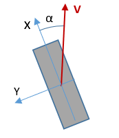
Understeer is the difference between the average front and rear tire slip angles.
For a neutral steer vehicle the slip angles will be the same, for an understeering
vehicle the front slip angles are of greater magnitude than the rear slip angles,
while for an oversteering vehicle the rear slip angles are of greater magnitude than
the front slip angles.
Here:
= Slip-angle: The angle in radians measured from the
velocity vector to the tire heading looking downward from above the tire. Figure 1.
The event can be run in lateral acceleration control mode or in velocity control mode. In
lateral acceleration control mode, the vehicle is driven at a constant speed around the
circular track, which results in a constant lateral acceleration.
In velocity control mode, the vehicle is driven at an increasing speed around the circular
path, which results in an increase in lateral acceleration. Using the event form, you can
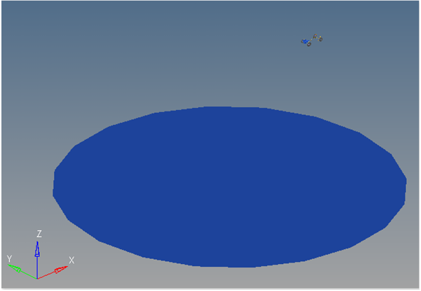
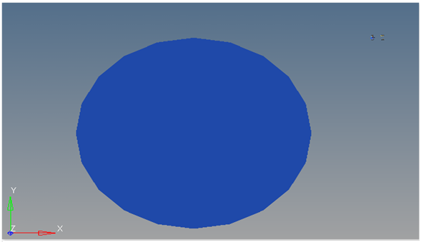
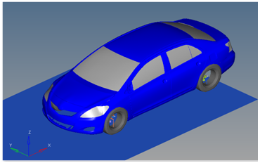
control the driving time, constant radius, and end speed. Figure 2. Constant Radius Event Figure 3. Top View of a Constant Radius Path Figure 4. Vehicle Model with Body Graphics
The event is designed to drive a vehicle on a constant radius at either a constant lateral
acceleration or at a steadily increasing speed. The event begins with a straight section of
road that allows the vehicle to come to steady state. The vehicle enters the turn and the
controllers maintain the desired velocity or lateral acceleration.
Lateral Acceleration Control
If lateral acceleration is selected for the vehicle control, the event is run at a steady
state lateral acceleration. A target lateral acceleration and the radius of the track are
entered in the form. The vehicle initial speed is calculated using the equation
v=sqrt(r*a). The equation is embedded in the form.
The event sequence is described in the table below:
Event Step
Description
Start
Vehicle begins driving in a straight line towards the constant radius circle tangent
at the speed that will generate a Lateral Acceleration that was entered in the
form.
Turn into Constant Radius Track
Vehicle enters the constant radius track. Turn direction is determined from the form
entry (left or right). Steering is controlled by the steer controller. Speed is
maintained by the drive torque controller. Lateral acceleration should be constant
(because speed is constant).
Follow the Constant Radius
The vehicle follows the constant radius path for the time defined in the event.
End of Event
The event ends when the time in circular track time is met.
A series of lateral acceleration control events is typically run to characterize the
vehicle. A series would include left and right turns (to understand the symmetry of the
vehicle) and a sweep of lateral accelerations to characterize the behavior of the vehicle as
acceleration increases. The track radius should match the radius of the test track being
used to generate correlation data.
Velocity Control
When the vehicle control is velocity, the vehicle drives around the track at a steadily
increasing speed and as a result, an increasing lateral acceleration. This event provides a
sweep of the lateral acceleration behavior of the vehicle (at increasing speeds). Left and
right turn directions can be run and the time in the circle can be varied to provide a
slower acceleration. The vehicle makes multiple loops around the circle if there is enough
time. The event sequence is shown in the table below.
Event Step
Description
Start
The vehicle drives toward the tangent of the Constant radius path. The initial speed
is determined from the Circle Radius and the desired initial Lateral Acceleration. Low
accelerations result in lower initial speeds.
Turn into Constant Radius Path
The vehicle turns into the Constant radius path and begins to accelerate.
Follow Constant Radius Path
The vehicle drives along the Constant radius path and increases speed. The vehicle
speed is increased from the initial speed to the final speed in the Time in circular
track time. Use a longer time to minimize acceleration effects on the results.
Event End
The event ends after the Time in circular track time is complete.
If the model cannot maintain the circular path, the error Could not Find
Ideal SWA in 20 Iterations is sent to the log file. This is a generic error
that indicates the path is not being followed. It can be caused by a wide variety of issues
with the model and the tires. Examine the model results at the time prior to the error being
displayed to understand what the vehicle may be doing.
Nine types of modeling element containers are used to define the event. Three sub-systems
(output requests, a steer controller, and a drive torque controller) are also included in
the event.
Datasets
One dataset is used in the system and it contains the data used to describe the Constant Radius event. The event allows you to set the vehicle control, lateral
acceleration, final vehicle velocity, time in the circular track, circle radius and turn
direction (left or right). The vehicle velocity, wheel rotational velocities and ground
height are calculated values and should not be changed.
Forms
The form is the only place that you should change the lane change event. circle radius,
turn direction, time in the circular track, vehicle control, lateral acceleration and final
vehicle velocity are the parameters that can be changed. The ground z coordinate and initial
vehicle velocity are calculated values. The ground z coordinate is calculated using the
wheel CG Z location and the tire rolling radius from the tire data.
Graphics
One graphic is defined in the event. The graphics define the road surface graphics and
should not require any user input. A full description of the graphics can be found here.
Skidpad graphics are included to illustrate the path being driven, and are defined
parametrically using the data in the Constant Radius event form. Skidpad
graphics should never require editing unless the event is being fundamentally changed. Figure 5. Skidpad Graphics
Joints
A ball joint is included in the Constant Radius event. The joint attaches a
dummy body to the steering rack. The joint is included to make certain events work in ADAMS.
Attach the dummy body to the steering rack if building a model manually.
Markers
One marker is included in the Constant Radius event. The path origin is the
origin of skidpad graphics and is parametrically defined to be the CG of the vehicle body.
The markers refer to points, and the points contain the parametric logic.
Motions
Three motions are included in the event. The steering motion to the vehicle is provided by
the steer controller and acts on a revolute joint that connects the steering column to the
vehicle body. If a steering column is not included in the model, the joint acts between the
steering rack input shaft and the vehicle body.
The front and rear wheel motions act on the wheel spindle revolute joints that connect the
wheel hub to the knuckle. The motion is initially zero (fixing the wheels to the knuckle) so
the model converges statically. The motions are deactivated after the static equilibrium
analysis to allow the tires to rotate.
Points
Two points are defined in the event. All points are used to create the skidpad graphics.
The points contain parametric logic to define their X, Y, and Z locations. You should not
need to modify any points.
Solver Variables
The Constant Radius event consists of only one solver variable, the Steer Path
Variable, which calls a user subroutine to apply an input at the steering wheel in order to
follow a desired path.
The numbers in the solver variable USER subroutine call are as follows:
Number
Description
5020
Branching ID. 5020 is a Constant radius event.
70000000
The ID of a solver array containing Driver Model Controller data. The array is in
the steer controller system.
70000100
The ID of a Vehicle Data array containing vehicle information. The array is in the
steer controller system.
30
The value of the circle radius.
Templates
A template is included in the Constant Radius event task. The template is
solver specific, and only the MotionSolve template is
documented. The template is inserted in the solver deck after the </Model>
command and controls the execution of the event.

 = Slip-angle: The angle in radians measured from the
velocity vector to the tire heading looking downward from above the tire.
= Slip-angle: The angle in radians measured from the
velocity vector to the tire heading looking downward from above the tire.