General Degenerated 4-Node Shell Formulations

Notational Conventions

• A bold letter denotes a vector or a tensor.
• An upper case index denotes a node number; a lower case index denotes a component of vector or tensor.
• The Einstein convention applies only for the repeated index where one is subscript and another is superscript, e.g.:

  $N_I{x}^I={\displaystyle \sum N_I{x}^I}$

• {} denotes a vector and [ ] denotes a matrix.

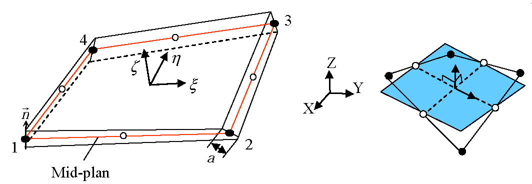
Geometry and Kinematics

Figure 1. Coordinate Systems

with $z=\frac{a\zeta }{2}$

with $\left[F_0\right]=\left[\left\{g_1\right\}\left\{g_2\right\}\frac{a}{2}\left\{n\right\}\right];g_1\left(\xi ,\eta \right)=X_{p,\xi }=N_{I,\xi }{X}^I,g_2\left(\xi ,\eta \right)=X_{p,\eta }=N_{I,\eta }{X}^I$

$F$ is the gradient tensor which is related to the Jacobian tensor $\left[J\right]={\left[F\right]}^t$ .

Where, $\beta$ and $\omega$ are the rotational velocity vectors of the normal: $\beta ={\beta }_1{t}_1+{\beta }_2{t}_2={\omega }_2{t}_1-{\omega }_1{t}_2$

and $\left(t_1,t_2,n\right)$ is base of the local coordinate system.

Equation 5 can be written also by:

$v_i=N_I{v}_i^I+z\left(-N_I{\omega }_1^I{t}_{2i}^I+N_I{\omega }_2^I{t}_{1i}^I\right);i=1,3$

This velocity interpolation is expressed in the global system, but ${\omega }^I$ must be defined first in the local nodal coordinate system to ensure Mindlin's kinematic condition.

Strain-Rate Construction

The in-plane rate-of-deformation is interpolated by the usual displacement method.

with $\left[Q\right]=\left[\left\{t_1\right\}\left\{t_2\right\}\left\{n\right\}\right]$ .

The Reissner-Mindlin conditions ${\epsilon }_{\zeta }=0$ and ${\sigma }_{\zeta }=0$ requires that the strain and stress tensors are computed in the local coordinate system (at each quadrature point).

After the linearization of $L_t$ with respect to $z$ , the in-plane rate-of-deformation terms are given by:

${\left[L_t\right]}_{2\times 2}=\left[L_{s0}\right]+z\left[L_{s1}\right]$

with the membrane terms:

$\left[L_{s0}\right]=\left[C_1\right]\left[C_0\right]$

The curvature-translation coupling is presented in the bending terms for a warped element (the first two terms in the last equation.)

The out-plane rate-of-deformation (transverse shear) is interpolated by the "assumed strain" method, which is based on the Hu-Washizu variation principle.

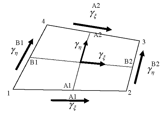
Where, ${\gamma }_{\xi }{}^{A\alpha },{\gamma }_{\eta }{}^{B\alpha }$ are the values of the covariant components at 4 mid-side points which vanish under a constant bending moment (Figure 2).

Figure 2. Covariant Components at 4 Mid-Side

Special Case for One-point Quadrature and the Difficulties in Stabilization

The formulations described above are general for both the full integration and reduced integration schemes. For a one-point quadrature element, you have the following particularities:

Where, $h_I=\left(\begin{array}{cccc}1& -1& 1& -1\end{array}\right)$ .

This implies that all the terms computed at the quadrature point are the constant parts with respect to $\left(\xi ,\eta \right)$ , and the stabilizing terms (hourglass) are the non-constant parts.

It would be ideal if the integration term $f_{stab}^{\mathrm{int}}$ could be evaluated explicitly. But such is not the case, and the main obstacles are the following:

For a non-coplanar element, the normal varies at each point so that it is difficult to write the non-constant part of strains explicitly. For a physically nonlinear problem, the non-constant part of stress is not generally in an explicit form. Thus, simplification becomes necessary.