Beam Elements (TYPE3)

Radioss uses a shear beam theory or Timoshenko formulation for its beam elements.

This formulation assumes that the internal virtual work rate is associated with the axial, torsional and shear strains. The other assumptions are:
  • No cross-section deformation in its plane.
  • No cross-section warping out of its plane.

With these assumptions, transverse shear is taken into account.

This formulation can degenerate into a standard Euler-Bernoulli formulation (the cross section remains normal to the beam axis). This choice is under user control.

Local Coordinate System

The properties describing a beam element are all defined in a local coordinate system.

This coordinate system can be seen in Figure 1. Nodes 1 and 2 of the element are used to define the local X axis, with the origin at node 1. The local Y axis is defined using node 3, which lies in the local XY plane, along with nodes 1 and 2. The Z axis is determined from the vector cross product of the positive X and Y axes.

The local Y direction is first defined at time t = 0 MathType@MTEF@5@5@+= feaagKart1ev2aaatCvAUfeBSjuyZL2yd9gzLbvyNv2CaerbuLwBLn hiov2DGi1BTfMBaeXatLxBI9gBaerbd9wDYLwzYbItLDharqqtubsr 4rNCHbGeaGqiVu0Je9sqqrpepC0xbbL8F4rqqrFfpeea0xe9Lq=Jc9 vqaqpepm0xbba9pwe9Q8fs0=yqaqpepae9pg0FirpepeKkFr0xfr=x fr=xb9adbaqaaeGaciGaaiaabeqaamaabaabaaGcbaGaamiDaiabg2 da9iaaicdaaaa@38AF@ and its position is corrected at each cycle, taking into account the mean rotation of the X axis. The Z axis is always orthogonal to the X and Y axes.

Deformations are computed with respect to the local coordinate system displaced and rotated to take into account rigid body motion. Translational velocities V MathType@MTEF@5@5@+= feaagKart1ev2aaatCvAUfeBSjuyZL2yd9gzLbvyNv2CaerbuLwBLn hiov2DGi1BTfMBaeXatLxBI9gBaerbd9wDYLwzYbItLDharqqtubsr 4rNCHbGeaGqiVu0Je9sqqrpepC0xbbL8F4rqqrFfpeea0xe9Lq=Jc9 vqaqpepm0xbba9pwe9Q8fs0=yqaqpepae9pg0FirpepeKkFr0xfr=x fr=xb9adbaqaaeGaciGaaiaabeqaamaabaabaaGcbaGaamOvaaaa@36D1@ and angular velocities Ω with respect to the global reference frame are expressed in the local frame.


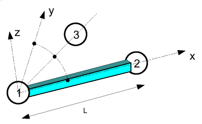
Figure 1. Beam Element Local Axis

Beam Element Geometry

The beam geometry is user-defined by:
A MathType@MTEF@5@5@+= feaagKart1ev2aaatCvAUfeBSjuyZL2yd9gzLbvyNv2CaerbuLwBLn hiov2DGi1BTfMBaeXatLxBI9gBaerbd9wDYLwzYbItLDharqqtubsr 4rNCHbGeaGqiVu0Je9sqqrpepC0xbbL8F4rqqrFfpeea0xe9Lq=Jc9 vqaqpepm0xbba9pwe9Q8fs0=yqaqpepae9pg0FirpepeKkFr0xfr=x fr=xb9adbaqaaeGaciGaaiaabeqaamaabaabaaGcbaGaamyqaaaa@36BC@
Cross section area
I x
Area moment of inertia of cross section about local x axis
I y
Area moment of inertia of cross section about local y axis
I z
Area moment of inertia of cross section about local z axis
The area moments of inertia about the y and z axes are concerned with bending. They can be calculated using the relationships:(1) I y = A z 2 d y d z (2) I z = A y 2 d y d z
The area moment of inertia about the x axis concerns torsion. This is simply the summation of the previous two moments of Ontario:(3) I x = I y + I z

Minimum Time Step

The minimum time step for a beam element is determined using the following relation:(4) Δt= aL c

Where,

c is the speed of sound: E / ρ ,

a = 1 2 min ( min ( 4 , 1 + b 12 ) F 1 , b 3 F 2 ) ,

F 1 = 1+2 d 2 2 d

F 2 =min( F 1 , 1+2 d s 2 2 d s )

b= A L 2 max( I y , I z )

d = max ( d m , d f )

d s =dmax( 1, 12 b 1+ 12E 5 6 Gb (1 I shear ) )

Beam Element Behavior

Radioss beam elements behave in four individual ways:
  • Membrane or axial deformation
  • Torsion
  • Bending about the z axis
  • Bending about the y axis

Membrane Behavior

Membrane or axial behavior is the extension or compression of the beam element. The forces acting on an element are shown in Figure 2.


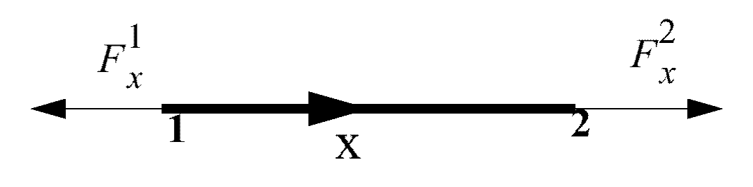
Figure 2. Membrane Forces
The force rate vector for an element is calculated using the relation:(5) [ F ˙ x 1 F ˙ x 2 ] = E A l [ + 1 1 1 + 1 ] [ υ x 1 υ x 2 ]
Where,
E
Elastic modulus
l
Beam element length
υ x
Nodal velocity in x direction
With the force rate equation, the force vector is determined using explicit time integration:(6) F x ( t+Δt )= F x ( t )+ F ˙ x Δt

Torsion

Torsional deformation occurs when the beam is loaded with a moment M about the X axis as shown in Figure 3.


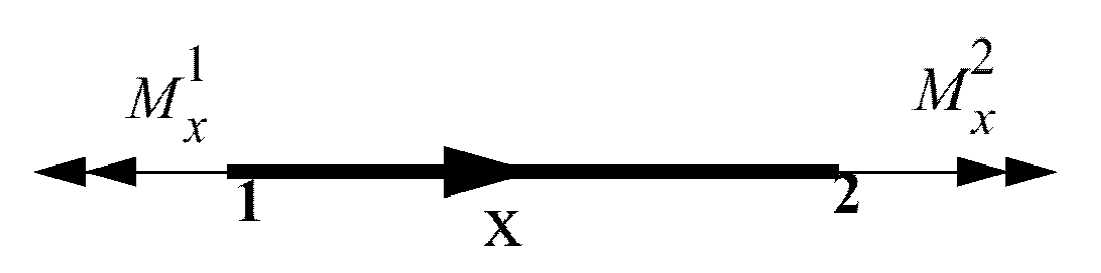
Figure 3. Torsional Loading
The moment rate vector is computed by:(7) [ M ˙ x 1 M ˙ x 2 ] = G I x l [ + 1 1 1 + 1 ] [ θ ˙ x 1 θ ˙ x 2 ]
Where,
G
Modulus of rigidity
θ ˙ x
Angular rotation rate
The moment about the X axis is found by explicit time integration:(8) M x ( t+Δt )= M x ( t )+ M ˙ x Δt

Bending About Z-axis

Bending about the z axis involves a force in the y direction and a moment about the z axis as shown in Figure 4.


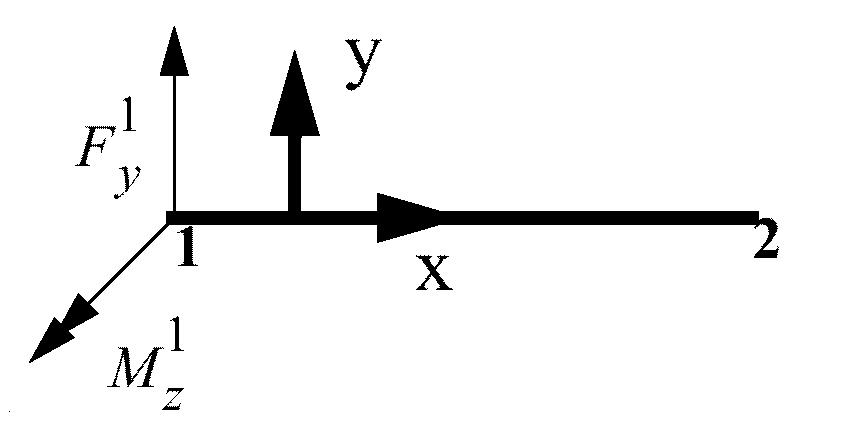
Figure 4. Bending about the Z Axis
Two vector fields must be solved for forces and moments. The rate equations are:(9) [ F ˙ y 1 F ˙ y 2 ] = E I z l 3 ( 1 + ϕ y ) [ + 12 6 l 12 + 6 l 12 6 l + 12 6 l ] [ v y 1 θ ˙ z 1 v y 2 θ ˙ z 2 ] (10) [ M ˙ z 1 M ˙ z 2 ] = E I z l 3 ( 1 + ϕ y ) [ + 6 l ( 4 + ϕ y ) l 2 6 l ( 2 ϕ y ) l 2 + 6 l ( 2 ϕ y ) l 2 6 l ( 4 + ϕ y ) l 2 ] [ v y 1 θ ˙ z 1 v y 2 θ ˙ z 2 ]

Where,

ϕ y = 144( 1+v ) I z 5A l 2 ,

υ is the Poisson's ratio.

The factor ϕ y MathType@MTEF@5@5@+= feaagKart1ev2aaatCvAUfeBSjuyZL2yd9gzLbvyNv2CaerbuLwBLn hiov2DGi1BTfMBaeXatLxBI9gBaerbd9wDYLwzYbItLDharqqtubsr 4rNCHbGeaGqiVu0Je9sqqrpepC0xbbL8F4rqqrFfpeea0xe9Lq=Jc9 vqaqpepm0xbba9pwe9Q8fs0=yqaqpepae9pg0FirpepeKkFr0xfr=x fr=xb9adbaqaaeGaciGaaiaabeqaamaabaabaaGcbaGaeqy1dy2aaS baaSqaaiaadMhaaeqaaaaa@38E8@ takes into account transverse shear.

The time integration for both is:(11) F y ( t + Δ t ) = F y ( t ) + F ˙ y Δ t (12) M z ( t + Δ t ) = M z ( t ) + M ˙ z Δ t

Bending About Y-axis

Bending about the Y axis is identical to bending about the Z axis. A force in the Y direction and a moment about the Z axis, shown in Figure 5, contribute to the elemental bending.


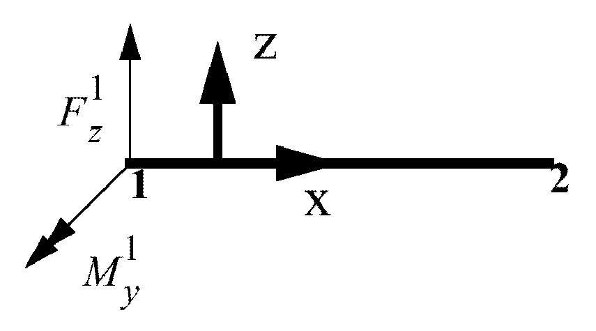
Figure 5. Bending about Y Axis
The rate equations are:(13) [ F ˙ z 1 F ˙ z 2 ] = E l y l 3 ( 1 + Φ z ) [ + 12 12 6 l 6 l 12 + 12 + 6 l 6 l ] [ ν z 1 θ ˙ y 1 ν z 2 θ ˙ y 2 ] (14) [ M ˙ y 1 M ˙ y 2 ] = E l y l 3 ( 1 + Φ z ) [ + 6 l + 6 l ( 4 + Φ z ) l 2 ( 2 Φ z ) l 2 6 l 6 l ( 2 Φ z ) l 2 ( 4 + Φ z ) l 2 ] [ ν z 1 θ ˙ y 1 ν z 2 θ ˙ y 2 ]

Where, Φ z = 144 ( 1 + ν ) I y 5 A l 2 .

Like bending about the Z axis, the factor Φ z introduces transverse shear.

With the time integration, the expression is:(15) F z ( t + Δ t ) = F z ( t ) + F ˙ z Δ t (16) M y ( t + Δ t ) = M y ( t ) + M ˙ y Δ t

Material Properties

A beam element may have two different types of material property:
  • Elastic
  • Elasto-plastic

Elastic Behavior

The elastic beam is defined using material LAW1 which is a simple linear material law.

The cross-section of a beam is defined by its area A MathType@MTEF@5@5@+= feaagKart1ev2aaatCvAUfeBSjuyZL2yd9gzLbvyNv2CaerbuLwBLn hiov2DGi1BTfMBaeXatLxBI9gBaerbd9wDYLwzYbItLDharqqtubsr 4rNCHbGeaGqiVu0Je9sqqrpepC0xbbL8F4rqqrFfpeea0xe9Lq=Jc9 vqaqpepm0xbba9pwe9Q8fs0=yqaqpepae9pg0FirpepeKkFr0xfr=x fr=xb9adbaqaaeGaciGaaiaabeqaamaabaabaaGcbaGaamyqaaaa@36BC@ and three area moments of inertia I x , I y and I z .

An elastic beam can be defined with these four parameters. For accuracy and stability, the following limitations should be respected:(17) L > A (18) 0.01 A 2 < I y < 100 A 2 (19) 0.01 A 2 < I z < 100 A 2 (20) 0.1 ( I y + I z ) < I x < 10 ( I y + I z )

Elasto-plastic Behavior

A global plasticity model is used.

The main assumption is that the beam cross section is full and rectangular. Optimal relations between sections and section inertia are:(21) 12 I y I z = A 4 (22) I x = I y + I z

However, this model also gives good results for the circular or ellipsoidal cross-section. For tubular or H cross-sections, plasticity will be approximated.

Recommendations:(23) L > A (24) 0.1 A 4 < 12 I y I z < 10 A 4 (25) 0.01 < I y / I z < 100 (26) 0.5 ( I y + I z ) < I x < 2 ( I y + I z )

Global Beam Plasticity

The elasto-plastic beam element is defined using material LAW2:(27) σ y = ( A + B ε p n ) ( 1 + C ln ε ˙ ε ˙ 0 )
The increment of plastic strain is:(28) Δ ε p = Δ W p l a s t i c σ y
The equivalent strain rate is derived from the total energy rate:(29) ε ˙ = Δ W t o t a l σ e q Δ t
Yield stress:(30) σ e q = F x 2 A 2 + 3 A ( M x 2 I x x + M y 2 I y y + M z 2 I z z )
If σ e q > σ y , you perform a radial return on the yield surface:(31) F x p a = F x σ y σ e q
and for i MathType@MTEF@5@5@+= feaagKart1ev2aaatCvAUfeBSjuyZL2yd9gzLbvyNv2CaerbuLwBLn hiov2DGi1BTfMBaeXatLxBI9gBaerbd9wDYLwzYbItLDharqqtubsr 4rNCHbGeaGqiVu0Je9sqqrpepC0xbbL8F4rqqrFfpeea0xe9Lq=Jc9 vqaqpepm0xbba9pwe9Q8fs0=yqaqpepae9pg0FirpepeKkFr0xfr=x fr=xb9adbaqaaeGaciGaaiaabeqaamaabaabaaGcbaGaamyAaaaa@36E4@ = x, y, z:(32) M i p a = M i σ y σ e q

Inertia Computation

The computational method of inertia for some kinds of elements as beam is particular as the inertia has to be transferred to the extremities of the beam. The nodal inertias are computed in function of the material density ρ , the cross-section area S MathType@MTEF@5@5@+= feaagKart1ev2aaatCvAUfeBSjuyZL2yd9gzLbvyNv2CaerbuLwBLn hiov2DGi1BTfMBaeXatLxBI9gBaerbd9wDYLwzYbItLDharqqtubsr 4rNCHbGeaGqiVu0Je9sqqrpepC0xbbL8F4rqqrFfpeea0xe9Lq=Jc9 vqaqpepm0xbba9pwe9Q8fs0=yqaqpepae9pg0FirpepeKkFr0xfr=x fr=xb9adbaqaaeGaciGaaiaabeqaamaabaabaaGcbaGaam4uaaaa@36CE@ , the element length L MathType@MTEF@5@5@+= feaagKart1ev2aaatCvAUfeBSjuyZL2yd9gzLbvyNv2CaerbuLwBLn hiov2DGi1BTfMBaeXatLxBI9gBaerbd9wDYLwzYbItLDharqqtubsr 4rNCHbGeaGqiVu0Je9sqqrpepC0xbbL8F4rqqrFfpeea0xe9Lq=Jc9 vqaqpepm0xbba9pwe9Q8fs0=yqaqpepae9pg0FirpepeKkFr0xfr=x fr=xb9adbaqaaeGaciGaaiaabeqaamaabaabaaGcbaGaam4uaaaa@36CE@ and the moments of inertia I x x , I y y , I z z :(33) M A X ( ( ρ S L 2 ) ( L 2 12 ) + ( ρ L 2 ) M A X ( I y y ; I z z ) ; ( ρ L 2 ) I x x )