General spring elements are defined as TYPE8 element property. They are mathematical elements,
which have 6 DOF, three translational displacements and three rotational degrees of freedom.
Each DOF is completely independent from the others. Spring displacements refer to either spring
extension or compression. The stiffness is associated to each DOF. Directions can either be
global or local. Local directions are defined with a fixed or moving skew frame. Global force
equilibrium is respected, but without global moment equilibrium. Therefore, this type of spring
is connected to the laboratory that applies the missing moments, unless the two defining nodes
are not coincident.
Time Step
The time step calculation for general spring elements is the same as the calculation of the
equivalent TYPE4 spring (Time Step).
Linear Spring
See Linear Spring; the explanation is the same as for spring TYPE4.
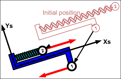
To help understand the use of skew frames, the deformation in the local x direction of the spring
will be considered. If the skew frame is fixed, deformation in the local X direction is shown in
Figure 1: Figure 1. Fixed Skew Frame
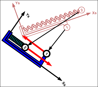
The same local x direction deformation, with a moving skew frame, can be seen in Figure 2. Figure 2. Moving Skew Frame
In both cases, the forces are in equilibrium, but the moments are not. If the first two nodes
defining the moving skew system are the same nodes as the two spring element nodes, the behavior
becomes exactly the same as that of a TYPE4 spring element. In this case the momentum
equilibrium is respected and local Y and Z deformations are always equal to zero.
Fixed Nodes
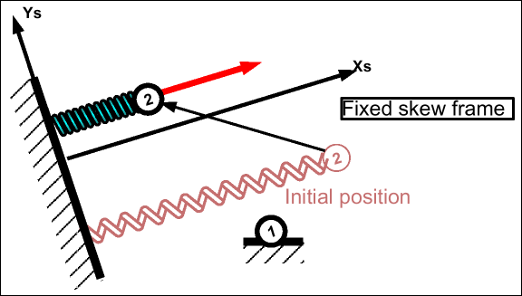
If one of the two nodes is completely fixed, the momentum equilibrium problem disappears. For
example, if node 1 is fixed, the force computation at node 2 is not dependent on the location of
node 1. The spring then becomes a spring between node 1 and the laboratory, as shown in Figure 3. Figure 3. Fixed Node - Fixed Skew Frame
It is generally recommended that a general spring element (TYPE8) be used only if one node is
fixed in all directions or if the two nodes are coincident. If the two nodes are coincident, the
translational stiffness' have to be large enough to ensure that the nodes remain near coincident
during the simulation.
Deformation Sign Convention
Positive and negative spring deformations are not defined with the variation of initial length. The initial length can be equal to zero for all or a given direction. Therefore, it is not possible to define the deformation sign with length variation.
The sign convention used is the following. A deformation is positive if displacement (or
rotation) of node 2 minus the displacement of node 1 is positive. The same sign convention is
used for all 6 degrees of freedom.(1)
(2)
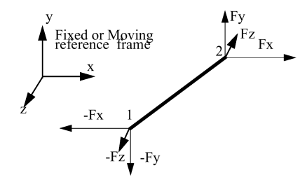
Translational Forces
The translational forces that can be applied to a general spring element can be seen in Figure 4. For each DOF (i = x, y, z), the force is calculated
by:(3)
Where,
Equivalent viscous damping coefficient
Force function related to spring displacement
The value of the displacement function depends on the type of general spring being modeled. Figure 4. Translational Forces
Linear Spring
If a linear general spring is being modeled, the translation forces are given
by:(4)
Where,
Stiffness or unloading stiffness (for elasto-plastic spring)
Nonlinear Spring
If a nonlinear general spring is being modeled, the translation forces are given
by:(5)
Where,
Function defining the change in force with spring displacement
Function defining the change in force with spring displacement rate
Coefficient
Default = 1
Coefficient
Coefficient
Default = 1
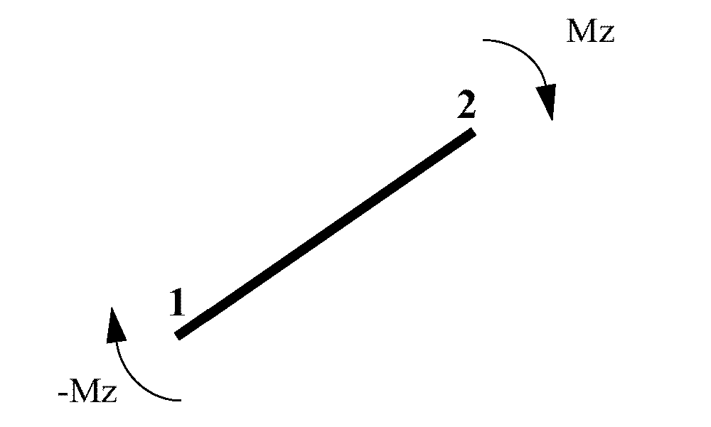
Moments
Moments can be applied to a general spring element, as shown in Figure 5. For each DOF (i = x, y, z), the moment is
calculated by:(6)
Where,
Equivalent viscous damping coefficient
Force function related to spring rotation
The value of the rotation function depends on the type of general spring being modeled. Not all
functions and coefficients defining moments and rotations are of the same value as that used in
the translational force calculation. Figure 5. General Spring Moments
Linear Spring
If a linear general spring is being modeled, the translation forces are given
by:(7)
Where,
Stiffness or unloading stiffness (for elasto-plastic spring)
Nonlinear Spring
If a nonlinear general spring is being modeled, the translation forces are given
by:(8)
Where,
Function defining the change in force with spring displacement
Function defining the change in force with spring displacement rate
Coefficient
Default = 1
Coefficient
Coefficient
Default = 1
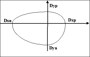
Multidirectional Failure
Criteria
Flag for rupture criteria: Ifail
Ifail=1
The rupture criteria flag is set to 1 in this case:(9)
Where,
The rupture displacement in positive x direction if
The rupture displacement in negative x direction if
Graphs of this rupture criterion can be seen in Figure 6. Figure 6. Multi-directional Failure Criteria Curves