One degree of freedom (DOF) spring elements are defined as a TYPE4 property set. Three variations
of the element are possible:
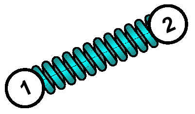
Spring only
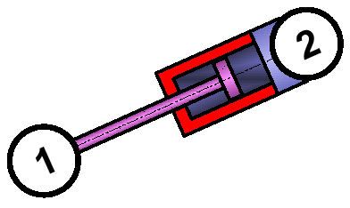
Dashpot (damper) only
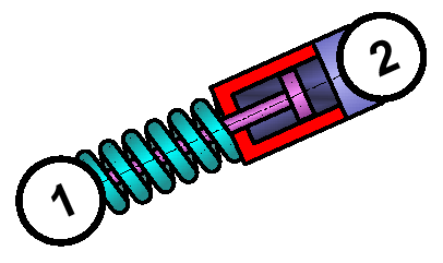
Spring and dashpot in parallel
These three configurations are shown in Figure 1 to Figure 3. Figure 1. Spring Only Figure 2. Dashpot Only Figure 3. Spring and Dashpot in Parallel
No material data card is required for spring elements. However, the stiffness and equivalent viscous damping coefficient are required. The mass is required if there is any spring translation.
There are three other options defining the type of spring stiffness with the hardening flag:
Linear Stiffness
Nonlinear Stiffness
Nonlinear Elasto-Plastic Stiffness
Likewise, the damping can be either:
Linear
Nonlinear
A spring may also have zero length. However, a one DOF spring must have 2 nodes.
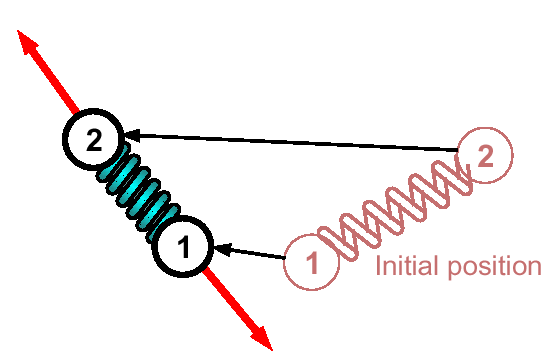
The forces applied on the nodes of a one DOF spring are always colinear with direction through
both nodes; refer to Figure 4. Figure 4. Colinear Forces
Time Step
The time of a spring element depends on the values of stiffness, damping and mass.
For a spring only element:(1)
For a dashpot only element:(2)
For a parallel spring and dashpot element:(3)
The critical time step ensures that the stability of the explicit time integration is
maintained, but it does not ensure high accuracy of spring vibration behavior. Only two time
steps are required during one vibration period of a free spring to keep stability. However, if
true sinusoidal reproduction is desired, the time step should be reduced by a factor of at least
5.
If the spring is used to connect the two parts, the spring vibration period increases and the
default spring time step ensures stability and accuracy.
Linear Spring
Function number defining .
N1=0
The general linear spring is defined by constant mass, stiffness and damping. These are all
required in the property type definition. The relationship between force and spring displacement
is given by:(4)
Figure 5. Linear Force-Displacement Curve
The stability condition is given by Equation 3:(5)
Nonlinear Elastic Spring
Hardening flag
H=0
The hardening flag must be set to 0 for a nonlinear elastic spring. The only difference
between linear and nonlinear elastic spring elements is the stiffness definition. The mass and
damping are defined as constant. However, a function must be defined that relates the force,
, to the displacement of the spring, (). It is defined as:(6)
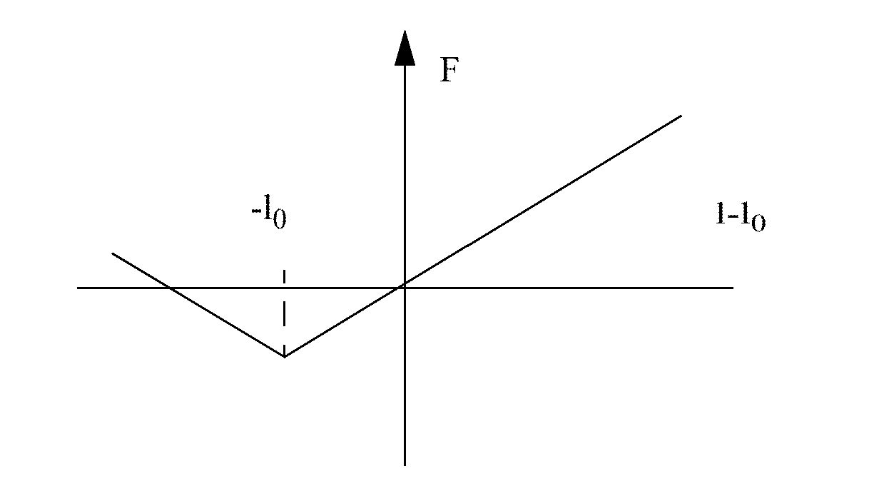
The hardening flag must be set to 1 in this case and is defined by a function. Hardening is isotropic if compression
behavior is identical to tensile behavior:(9)
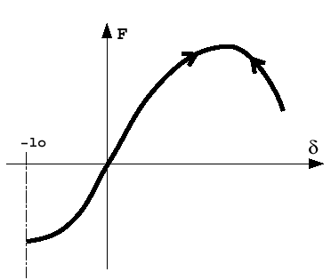
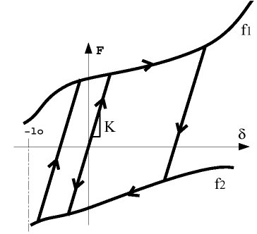
The hardening flag is set to 4 in this case and and (respectively maximum and minimum yield force) are defined by a
function. The hardening is kinematic if maximum and minimum yield curves are
identical:(11)
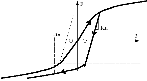
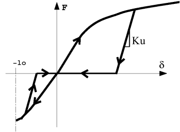
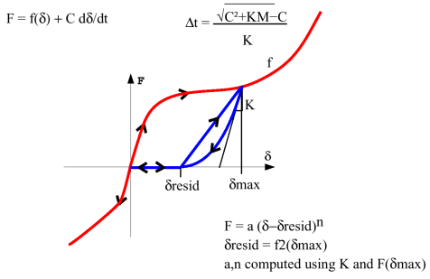
The hardening flag is set to 5 in this case and and (maximum yield force and residual deformation, respectively) are
defined by a function. Uncoupled hardening in compression and tensile behavior with nonlinear
unloading:(12)
With . Figure 10. Nonlinear Unloading Force-Displacement Curve
Nonlinear Dashpot
The input properties for a nonlinear dashpot are very close to that of a spring. The required
values are:
Mass, .
A function defining the change in force with respect to the spring displacement. This must
be equal to unity:
A function defining the change in force with spring displacement rate,
The hardening flag in the input must be set to zero.
The relationship between force and spring displacement and displacement rate
is:(13)
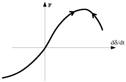
A nonlinear dashpot property is shown in Figure 11. Figure 11. Nonlinear Dashpot Force Curve
The stability condition for a nonlinear dashpot is given by:(14)
Where,(15)
Nonlinear Viscoelastic Spring
The input properties for a nonlinear viscoelastic spring are:
Mass,
Equivalent viscous damping coefficient
A function defining the change in force with spring displacement
A function defining the change in force with spring displacement rate
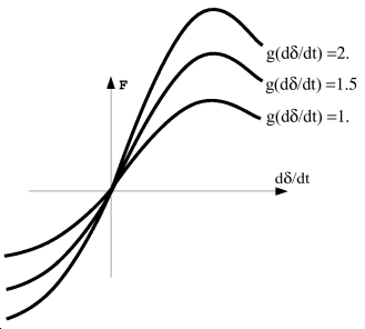
The hardening flag in the input must be set to equal zero. The force relationship is given
by:(16)
Graphs of this relationship for various values of are shown in Figure 12. Figure 12. Visco-Elastic Spring Force-Displacement Curves