Linear Stability

The stability of solution concerns the evolution of a process subjected to small perturbations. A process is considered to be stable if small perturbations of initial data result in small changes in the solution. The theory of stability can be applied to a variety of computational problems.

The numerical stability of the time integration schemes is widely discussed in the Theory Manual. Here, the stability of an equilibrium state for an elastic system is studied. The material stability will be presented in an upcoming version of this manual.

The stability of an equilibrium state is of considerable interest. It is determined by examining whether perturbations applied to that equilibrium state grow. A famous example of stable and unstable cases is often given in the literature. It concerns a ball deposited on three kinds of surfaces as shown in Figure 1.


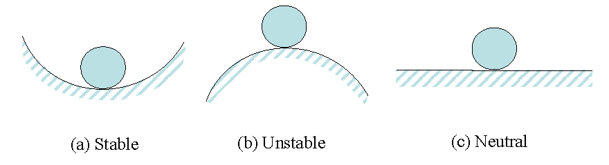
Figure 1. Schematic Presentation of Stability

It is clear that the state (b) represents an unstable case since a small change in the position of the ball results the rolling either to the right or to the left. It is worthwhile to mention here that stability and equilibrium notions are quite different. A system in static equilibrium may be in unstable state and a system in evolution is not necessary unstable.

A good understanding of the stability of equilibrium can be obtained by studying the load-deflection curves. A typical behavior of a structure in buckling is given in Figure 2. The load-deflection curves are slightly different for systems with and without imperfection. In the first case, the structure is loaded until the bifurcation point B corresponding to the first critical load level. Then, two solutions are mathematically acceptable: response without buckling (BA), response after buckling (BC).

In the case of structures with imperfection, no bifurcation point is observed. The behavior before buckling is not linear and the turning point D is the limit point in which the slope of the curve changes sign. If the behavior before buckling is linear or the nonlinearity before the limit point is not high, the linear stability technique can be used to determine the critical load. The method is based on the perturbation of the equilibrium state. As the perturbations are small, the linearized model is used. The method is detailed in the following section.


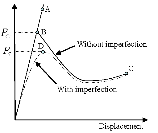
Figure 2. Bifurcation and Limit Points in Load-Deflection Curves for System With and Without Imperfections. B: Bifurcation point, D: Limit point

General Theory of Linear Stability

The principle of virtual power and the minimum of total potential energy are the various mathematical models largely used in Finite Element Method. Under small-perturbations assumption these notions can be applied to the equilibrium state in order to study the stability of the system.

Consider the example of the ball on the three kinds of surfaces as shown in Linear Stability, Figure 1. If Π is the total potential energy, the equilibrium is obtained by:
Static equilibrium
(1) δ Π = 0
Applying a small perturbation to the equilibrium state, the variation of the total potential energy can be written as:(2) δ Π ( t + Δ t ) = δ Π ( t ) + δ 2 Π
Where, δ 2 Π is the second variation of the potential energy. Then, the three cases can be distinguished:
Stable (case a)
(3) δ 2 Π > 0
The energy increases around the equilibrium state.
Unstable (case b)
(4) δ 2 Π < 0
The energy decreases around the equilibrium state.
Neutral stability (case c)
(5) δ 2 Π = 0
The energy remains unchanged around the equilibrium state.
The last case is used to compute the critical loads:(6) δ 2 Π = δ 2 Π int + δ 2 Π e x t = 0
Where, the indices int MathType@MTEF@5@5@+= feaagKart1ev2aaatCvAUfeBSjuyZL2yd9gzLbvyNv2CaerbuLwBLn hiov2DGi1BTfMBaeXatLxBI9gBaerbd9wDYLwzYbItLDharqqtubsr 4rNCHbGeaGqiVu0Je9sqqrpepC0xbbL8F4rqqrFfpeea0xe9Lq=Jc9 vqaqpepm0xbba9pwe9Q8fs0=yqaqpepae9pg0FirpepeKkFr0xfr=x fr=xb9adbaqaaeGaciGaaiaabeqaamaabaabaaGcbaGaciyAaiaac6 gacaGG0baaaa@38CF@ and ext MathType@MTEF@5@5@+= feaagKart1ev2aaatCvAUfeBSjuyZL2yd9gzLbvyNv2CaerbuLwBLn hiov2DGi1BTfMBaeXatLxBI9gBaerbd9wDYLwzYbItLDharqqtubsr 4rNCHbGeaGqiVu0Je9sqqrpepC0xbbL8F4rqqrFfpeea0xe9Lq=Jc9 vqaqpepm0xbba9pwe9Q8fs0=yqaqpepae9pg0FirpepeKkFr0xfr=x fr=xb9adbaqaaeGaciGaaiaabeqaamaabaabaaGcbaGaamyzaiaadI hacaWG0baaaa@38D6@ denote the interval and external parts of the total potential energy. After the application of the application of finite element method, the stability equation in a discrete form can be written as:(7) δ 2 Π = n δ 2 Π int e + n δ 2 Π e x t e = 0 (8) δ 2 Π e x t e = S e 0 δ X { δ f n } d S e 0 (9) δ 2 Π int e = V e 0 ( [ E ] [ S ] + [ δ E ] [ δ S ] ) d V e 0
Where,
e MathType@MTEF@5@5@+= feaagKart1ev2aaatCvAUfeBSjuyZL2yd9gzLbvyNv2CaerbuLwBLn hiov2DGi1BTfMBaeXatLxBI9gBaerbd9wDYLwzYbItLDharqqtubsr 4rNCHbGeaGqiVu0Je9sqqrpepC0xbbL8F4rqqrFfpeea0xe9Lq=Jc9 vqaqpepm0xbba9pwe9Q8fs0=yqaqpepae9pg0FirpepeKkFr0xfr=x fr=xb9adbaqaaeGaciGaaiaabeqaamaabaabaaGcbaGaamyzaaaa@36E0@
Designate element
{ f n }
Vector of the external forces
δ X
Virtual displacement vector
[ E ]
Green-Lagrange strain tensor
[ S ]
Piola-Kirchhoff stress tensor

The equation Equation 9 is written as a function of X, the displacement between the initial configuration C 0 and the critical state C t . If X L and S L are the linear response obtained after application the load f L in the initial configuration C 0 , in linear theory of stability suppose that the solution in C t for the critical load f c r is proportional to the linear response:

{ X c r } = λ { X L } (10) { S c r } = λ { S L }

{ F c r } = λ { F L }

If you admit that the loading does not depend on the deformation state, the hypothesis δ 2 Π e x t = 0 is then true. Using Kinematic Description, Equation 23 and denoting [ e ] for the linear part of Green-Lagrange strain tensor and [ η ] for the nonlinear part, you have:(11) { E } = { e } + { η }
Putting this equation in Equation 9, you obtain:(12) δ 2 Π e e x t = V 0 e ( δ e [ C ] { δ e } + λ ( δ η L [ C ] { δ e } + δ e [ C ] [ δ η L ] + S { δ 2 E } ) ) d V e 0
Or (13) δ 2 Π e e x t = δ X ( [ k ] + λ ( [ k u ( X L ) ] + [ k σ ] ) ) { δ X }
Where,
[ k ]
Stiffness matrix
[ k u ]
Initial displacement matrix
[ k σ ]
Initial stress or geometrical stiffness matrix
[ C ]
Elastic matrix
The linear theory of stability allows estimating the critical loads and their associated modes by resolving an eigenvalue problem:(14) ( [ K ] + λ ( [ K u ] + [ K σ ] ) ) { δ X } = 0

Linear stability assumes the linearity of behavior before buckling. If a system is highly nonlinear in the neighborhood of the initial state C 0 , moderate perturbations may lead to unstable growth. In addition, in case of path-dependent materials, the use of method is not conclusive from an engineering point of view. However, the method is simple and provides generally good estimations of limit points.

The resolution procedure consists in two main steps. First, the linear solution for the equilibrium of the system under the application of the load { F L } is obtained. Then, Equation 14 is resolved to compute the first desired critical loads and modes. The methods to compute the eigen values are those explained in Large Scale Eigen Value Computation.