Composite Shell Elements
- TYPE9 Element Property - Orthotropic Shell
- TYPE10 Element Property - Composite Shell
- TYPE11 Element Property - Composite Shell with variable layers
These elements are primarily used with the Tsai-Wu model (material LAW25). They allow one global behavior or varying characteristics per layer, with varying orthotropic orientations, varying thickness and/or varying material properties, depending on which element is used. Elastic, plastic and failure modeling can be undertaken.
Transformation Matrix: Global to Orthotropic Skew
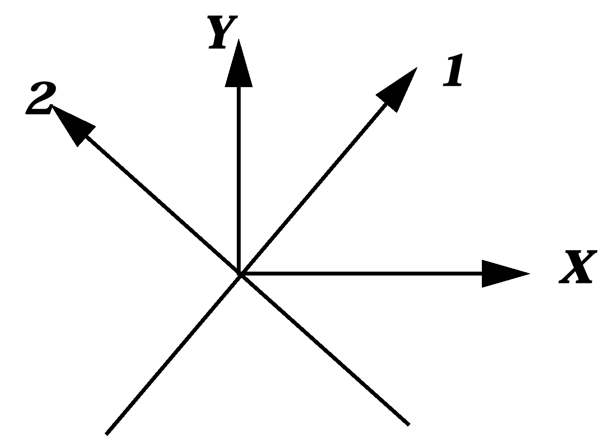
Figure 1. Fiber Orientation
Composite Modeling
Radioss has been successfully used to predict the behavior of composite structures for crash and impact simulations in the automotive, rail and aeronautical industries.
The purpose of this chapter is to present the various options available in Radioss to model composites, as well as some modeling methods.
Modeling Composites with Shell Elements
Composite materials with up to 100 layers may be modeled, each with different material properties, thickness, and fiber directions.
Lamina plasticity is taken into account using the Tsai-Wu criteria, which may also consider strain rate effects. Plastic work is used as a plasticity as well as rupture criterion.
Fiber brittle rupture may be taken into account in both orthotropic directions.
Delamination may be taken into account through a damage parameter in shear direction.
Modeling Composites with Solid Elements
Solid elements may be used for composites.
- Solid composite materials: one layer of composite is modeled with one solid element. Orthotropic characteristics and yield criteria are the same as shell elements (Modeling Composites with Shell Elements).
- A honeycomb material law is also available, featuring user defined yield curves for all components of the stress tensor and rupture strain.
Solid + Shell Elements
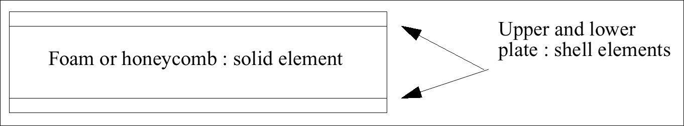
Figure 2.
Element Orientation
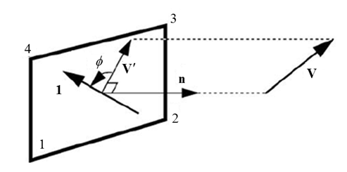
Figure 3. Fiber Direction Orientation
The shell normal defines the positive direction for . For elements with more than one layer, multiple angles can be defined.
- Constant orientation in local corotational reference frame constant orientation in local isoparametric frame. The first formulation may lead to unstable models especially in the case of very thin shells (airbag modeling). In Figure 4 the difference between the two formulations is illustrated for the case of element traction and shearing.
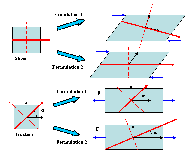
Figure 4. Fiber Direction Updating
Orthotropic Shells
- Only one layer
- Can have up to 5 integration points1 through the thickness
- One orientation
- One material property
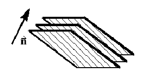
Figure 5.
Composite Shells
- Up to 100 layers can be modeled
- Constant layer thickness
- Constant reference vector
- Variable layer orientation
- Constant material properties
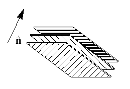
Figure 6.
Composite Shells with Variable Layers
- Up to 100 layers can be modeled
- Variable layer thicknesses
- Constant reference vector
- Variable layer orientation
- Variable material properties, mi2,3
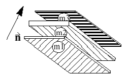
Figure 7.
Limitations
When modeling a composite material, there are two strategies that may be applied. The first, and simplest, is to model the material in a laminate behavior. This involves using TYPE9 property shell elements. The second is to model each ply of the laminate using one integration point. This requires either a TYPE10 or TYPE11 element.
Modeling using the TYPE9 element allows global behavior to be modeled. Input is simple, with only the reference vector as the extra information. A Tsai-Wu yield criterion and hardening law is easily obtained from the manufacturer or a test of the whole material.
Using the TYPE10 or TYPE11 element, one model's each ply in detail, with one integration point per ply and tensile failure is described in detail for each ply. However, the input requirements are complex, especially for the TYPE11 element.
Delamination is the separation of the various layers in a composite material. It can occur in situations of large deformation and fatigue. This phenomenon cannot be modeled in detail using shell theory. A global criterion is available in material LAW25. Delamination can affect the material by reducing the bending stiffness and buckling force.