Shell elements behave in two ways, either membrane or bending behavior. The Mindlin plate
elements that are used by Radioss account for bending and
transverse shear deformation. Hence, they can be used to model thick and thin plates.
Membrane Behavior
The membrane strain rates for Mindlin plate elements are defined as:(1)
(2)
(3)
(4)
(5)
Where,
Membrane strain rate
Bending Behavior
The bending behavior in plate elements is described using the amount of curvature. The
curvature rates of the Mindlin plate elements are defined as:(6)
(7)
(8)
Where,
Curvature rate
Strain Rate Calculation
The calculation of the strain rate of an individual element is divided into two parts,
membrane and bending strain rates.
Membrane Strain Rate
The vector defining the membrane strain rate is:(9)
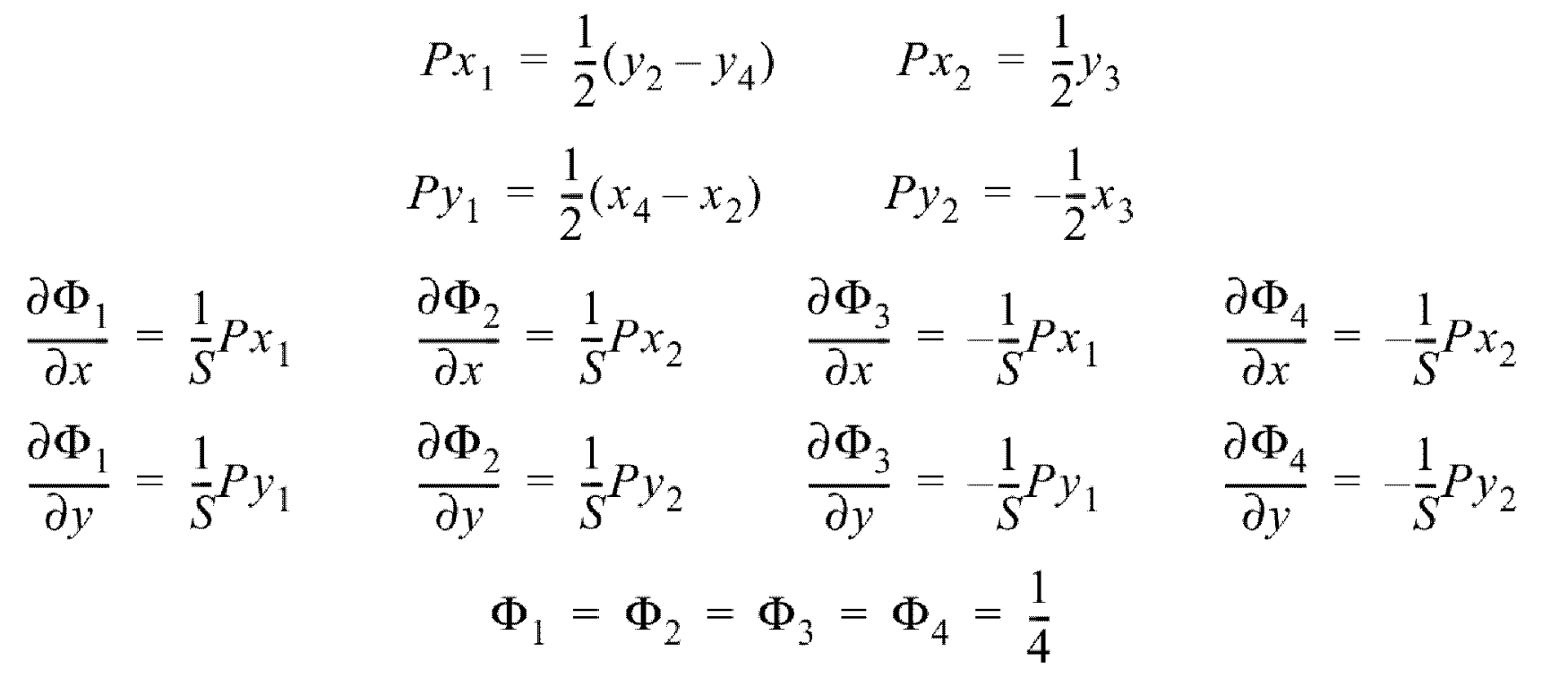
This vector is computed from the velocity field vector and the shape function gradient :(10)
Where,(11)
(12)
Bending Strain Rate
The vector defining the bending strain rate is:(13)
As with the membrane strain rate, the bending strain rate is computed from the
velocity field vector. However, the velocity field vector for the bending strain rate
contains rotational velocities, as well as translations:(14)
Where,(15)
(16)
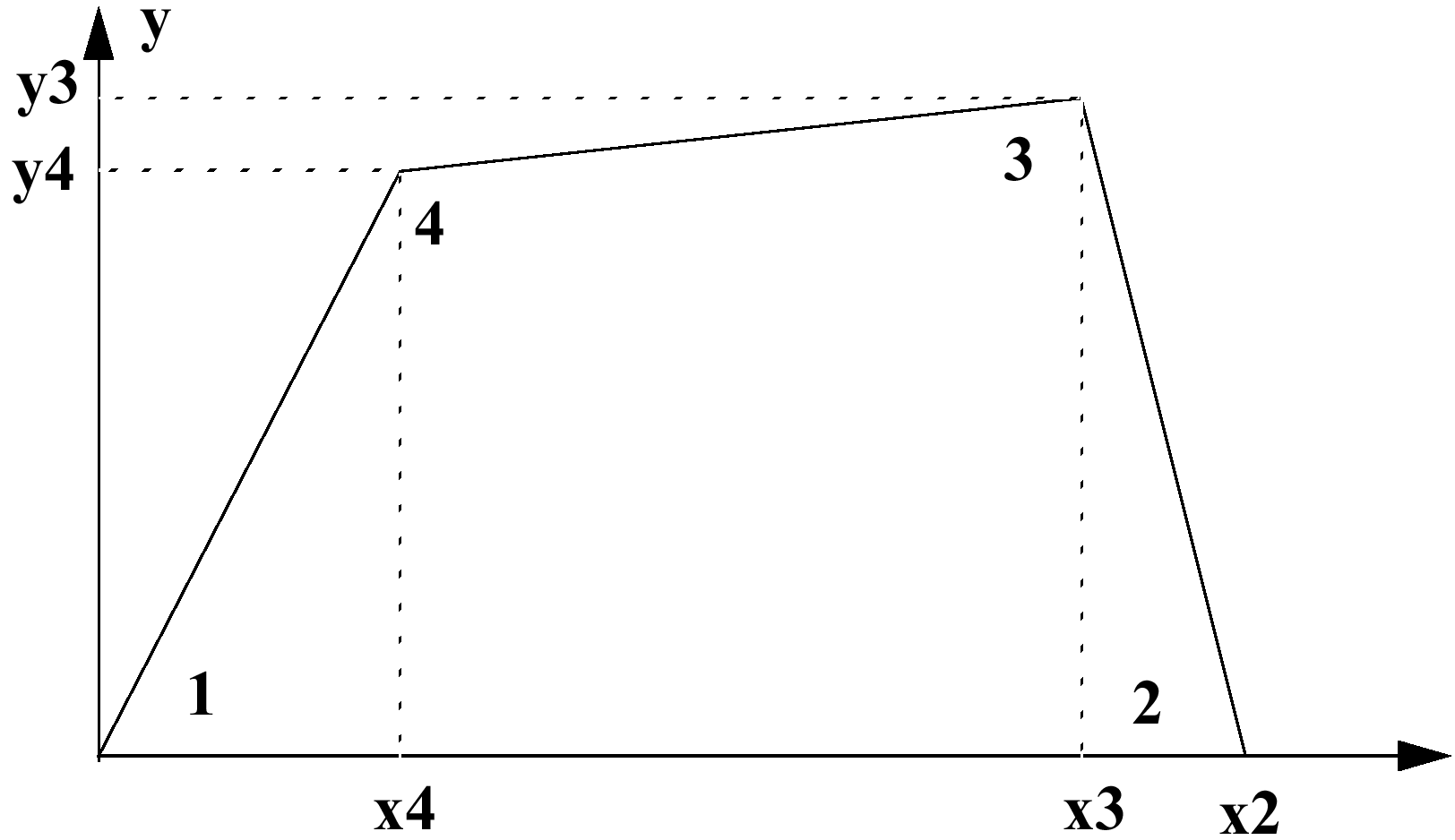
Figure 1. Strain Rate Calculation(17)
Mass and Inertia
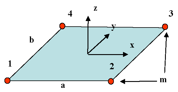
Consider a rectangular plate with sides of length and , surface area and thickness , as shown in Figure 2. Figure 2. Mass Distribution
Due to the lumped mass formulation used by Radioss, the lumped
mass at a particular node is:(18)
The mass moments of inertia, with respect to local element reference frame, are calculated
at node by:(19)
(20)
(21)
(22)
Inertia Stability
With the exact formula for inertia (Equation 19 to Equation 22), the solution tends to
diverge for large rotation rates. Belytschko proposed a way to stabilize the solution by
setting
=
, that is, to consider the rectangle as a square with respect
to the inertia calculation only. This introduces an error into the formulation. However, if
the aspect ratio is small the error will be minimal. In Radioss
a better stabilization is obtained by:(23)
(24)
(25)
Where, is a regulator factor with default value =12 for QBAT element and =9 for other quadrilateral elements.