3-Node Triangle without Rotational DOF

The need of simple and efficient element in nonlinear analysis of shells undergoing large rotations is evident in crash and sheet metal forming simulations. The constant-moment plate elements fit this need. One of the famous concepts in this field is that of Batoz et al. 1 known under DKT elements where DKT stands for Discrete Kirchhoff Triangle. The DKT12 element 1, 2 has a total of 12 DOFs. The discrete Kirchhoff plate conditions are imposed at three mid-point of each side. The element makes use of rotational DOF. at each edge to take into account the bending effects. A simplified three-node element without rotational DOF is presented in 3. The rotational DOF is computed with the help of out-of-plane translational DOF in the neighbor elements. This attractive approach is used in Radioss in the development of element SH3N6 which based on DKT12.

Strain Computation

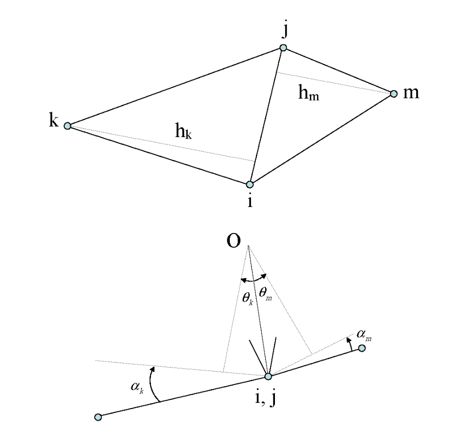
Consider two adjacent coplanar elements with a common edge i-j as shown in Figure 2. Due to out-of-plane displacements of nodes m MathType@MTEF@5@5@+= feaagKart1ev2aaatCvAUfeBSjuyZL2yd9gzLbvyNv2CaerbuLwBLn hiov2DGi1BTfMBaeXatLxBI9gBaerbd9wDYLwzYbItLDharqqtubsr 4rNCHbGeaGqiVu0Je9sqqrpepC0xbbL8F4rqqrFfpeea0xe9Lq=Jc9 vqaqpepm0xbba9pwe9Q8fs0=yqaqpepae9pg0FirpepeKkFr0xfr=x fr=xb9adbaqaaeGaciGaaiaabeqaamaabaabaaGcbaGaamyBaaaa@36E8@ and k MathType@MTEF@5@5@+= feaagKart1ev2aaatCvAUfeBSjuyZL2yd9gzLbvyNv2CaerbuLwBLn hiov2DGi1BTfMBaeXatLxBI9gBaerbd9wDYLwzYbItLDharqqtubsr 4rNCHbGeaGqiVu0Je9sqqrpepC0xbbL8F4rqqrFfpeea0xe9Lq=Jc9 vqaqpepm0xbba9pwe9Q8fs0=yqaqpepae9pg0FirpepeKkFr0xfr=x fr=xb9adbaqaaeGaciGaaiaabeqaamaabaabaaGcbaGaamyBaaaa@36E8@ , the elements rotate around the side i-j. The angles between final and initial positions of the elements are respectively α m and α k for corresponding opposite nodes m MathType@MTEF@5@5@+= feaagKart1ev2aaatCvAUfeBSjuyZL2yd9gzLbvyNv2CaerbuLwBLn hiov2DGi1BTfMBaeXatLxBI9gBaerbd9wDYLwzYbItLDharqqtubsr 4rNCHbGeaGqiVu0Je9sqqrpepC0xbbL8F4rqqrFfpeea0xe9Lq=Jc9 vqaqpepm0xbba9pwe9Q8fs0=yqaqpepae9pg0FirpepeKkFr0xfr=x fr=xb9adbaqaaeGaciGaaiaabeqaamaabaabaaGcbaGaamyBaaaa@36E8@ and k MathType@MTEF@5@5@+= feaagKart1ev2aaatCvAUfeBSjuyZL2yd9gzLbvyNv2CaerbuLwBLn hiov2DGi1BTfMBaeXatLxBI9gBaerbd9wDYLwzYbItLDharqqtubsr 4rNCHbGeaGqiVu0Je9sqqrpepC0xbbL8F4rqqrFfpeea0xe9Lq=Jc9 vqaqpepm0xbba9pwe9Q8fs0=yqaqpepae9pg0FirpepeKkFr0xfr=x fr=xb9adbaqaaeGaciGaaiaabeqaamaabaabaaGcbaGaamyBaaaa@36E8@ . Assuming, a constant curvature for both of elements, the rotation angles θ m and θ k related to the bending of each element around the common side are obtained by:(1)
θ k = h k 2 R and θ m = h m 2 R
However, for total rotation you have:(2)
θ k + θ m = α k + α m
which leads to:(3)
θ k = ( α k + α m ) h k ( h k + h m ) and θ m = ( α k + α m ) h m ( h k + h m )


Figure 1. Computation of Rotational DOF in SH3N6
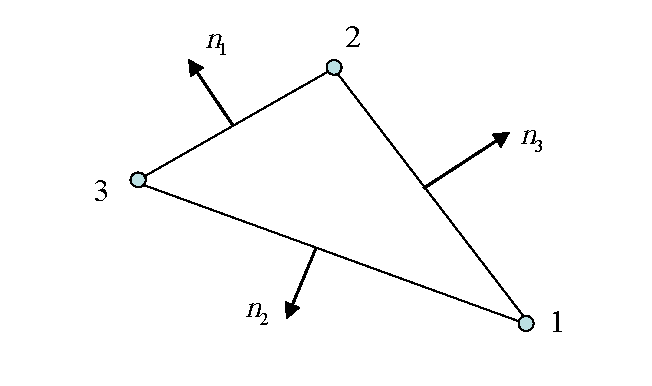
Consider the triangle element in Figure 2. The outward normal vectors at the three sides are defined and denoted n 1 MathType@MTEF@5@5@+= feaagKart1ev2aaatCvAUfeBSjuyZL2yd9gzLbvyNv2CaerbwvMCKf MBHbqefqvATv2CG4uz3bIuV1wyUbqedmvETj2BSbqefm0B1jxALjhi ov2DaebbnrfifHhDYfgasaacH8srps0lbbf9q8WrFfeuY=Hhbbf9v8 qqaqFr0xc9pk0xbba9q8WqFfea0=yr0RYxir=Jbba9q8aq0=yq=He9 q8qqQ8frFve9Fve9Ff0dmeaacaGacmGadaWaaiqacaabaiaafaaake GabaaVqiaad6gacaaIXaaaaa@3B54@ , n 2 MathType@MTEF@5@5@+= feaagKart1ev2aaatCvAUfeBSjuyZL2yd9gzLbvyNv2CaerbwvMCKf MBHbqefqvATv2CG4uz3bIuV1wyUbqedmvETj2BSbqefm0B1jxALjhi ov2DaebbnrfifHhDYfgasaacH8srps0lbbf9q8WrFfeuY=Hhbbf9v8 qqaqFr0xc9pk0xbba9q8WqFfea0=yr0RYxir=Jbba9q8aq0=yq=He9 q8qqQ8frFve9Fve9Ff0dmeaacaGacmGadaWaaiqacaabaiaafaaake GabaaVqiaad6gacaaIXaaaaa@3B54@ and n 3 MathType@MTEF@5@5@+= feaagKart1ev2aaatCvAUfeBSjuyZL2yd9gzLbvyNv2CaerbwvMCKf MBHbqefqvATv2CG4uz3bIuV1wyUbqedmvETj2BSbqefm0B1jxALjhi ov2DaebbnrfifHhDYfgasaacH8srps0lbbf9q8WrFfeuY=Hhbbf9v8 qqaqFr0xc9pk0xbba9q8WqFfea0=yr0RYxir=Jbba9q8aq0=yq=He9 q8qqQ8frFve9Fve9Ff0dmeaacaGacmGadaWaaiqacaabaiaafaaake GabaaVqiaad6gacaaIXaaaaa@3B54@ . The normal component strain due to the bending around the element side is obtained using plate assumption:(4)
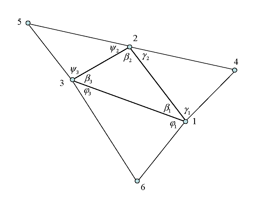
{ ε n 1 ε n 2 γ n 3 } = [ 2 ( h 1 + h 5 ) 0 0 0 2 ( h 1 + h 5 ) 0 0 2 ( h 2 + h 6 ) 0 0 0 2 ( h 2 + h 6 ) 0 0 2 ( h 3 + h 4 ) 2 ( h 3 + h 4 ) 0 0 ] { α 1 α 2 α 3 α 4 α 5 α 6 }
The six mid-side rotations α i are related to the out-of-plane displacements of the six apex nodes as shown in Figure 3 by the following relation:(5)
{ α 1 α 2 α 3 α 4 α 5 α 6 } = [ 1 h 1 cos β 3 h 2 cos β 2 h 3 0 0 0 cos β 3 h 1 1 h 2 cos β 1 h 3 0 0 0 cos β 2 h 1 cos β 1 h 2 1 h 3 0 0 0 cos γ 2 q 1 cos γ 1 q 2 0 1 h 4 0 0 0 cos ψ 3 r 2 cos ψ 2 r 3 0 1 h 5 0 cos φ 2 s 1 0 cos φ 1 s 3 0 0 1 h 6 ] { w 1 w 2 w 3 w 4 w 5 w 6 }
Where, ( h 1 h 2 h 3 ) , ( q 1 h 4 q 2 ) , ( r 2 h 5 r 3 ) and ( s 3 h 6 s 1 ) are respectively the heights of the triangles (1,2,3), (1,4,2), (2,5,3) and (3,6,1).


Figure 2. Normal Vectors Definition
The non-null components of strain tensor in the local element reference are related to the normal components of strain by the following relation: 1 3(6)
{ ε x x ε y y γ x y } = [ ( y 3 y 2 l 1 ) 2 ( y 1 y 3 l 2 ) 2 ( y 2 y 1 l 3 ) 2 ( x 2 x 3 l 1 ) 2 ( x 3 x 1 l 2 ) 2 ( x 1 x 2 l 3 ) 2 2 ( y 3 y 2 l 1 ) ( x 2 x 3 l 1 ) 2 ( y 1 y 3 l 2 ) ( x 3 x 1 l 2 ) 2 ( y 2 y 1 l 3 ) ( x 1 x 2 l 3 ) ] { ε n 1 ε n 2 γ n 3 }


Figure 3. Neighbor Elements for a Triangle

Boundary Conditions Application

As the side rotation of the element is computed using the out-of-plane displacement of the neighbor elements, the application of clamped or free boundary conditions needs a particular 
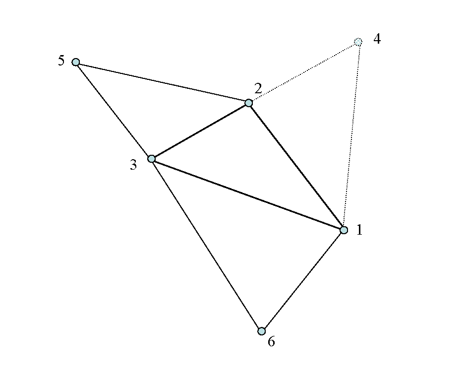
attention. It is natural to consider the boundary conditions on the edges by introducing a virtual and symmetric element outside of the edge as described in Figure 4. In the case of free rotation at the edge, the normal strain ε n k is vanished. From Equation 4, this leads to:(7)
α k = α m
In Equation 5 the fourth row of the matrix is then changed to:(8)
[ cos β 2 h 1 cos β 1 h 2 1 h 3 0 0 0 ]
The clamped condition is introduced by the symmetry in out-of-plane displacement, that is, w m = w k MathType@MTEF@5@5@+= feaagKart1ev2aaatCvAUfeBSjuyZL2yd9gzLbvyNv2CaerbwvMCKf MBHbqefqvATv2CG4uz3bIuV1wyUbqedmvETj2BSbqefm0B1jxALjhi ov2DaebbnrfifHhDYfgasaacH8srps0lbbf9q8WrFfeuY=Hhbbf9v8 qqaqFr0xc9pk0xbba9q8WqFfea0=yr0RYxir=Jbba9q8aq0=yq=He9 q8qqQ8frFve9Fve9Ff0dmeaacaGacmGadaWaaiqacaabaiaafaaake aacaWG3bWaaSbaaSqaaiaad2gaaeqaaOGaeyypa0Jaam4DamaaBaaa leaacaWGRbaabeaaaaa@3E19@ . This implies α k = α m . The fourth row of the matrix in Equation 5 is then changed to:(9)
[ cos β 2 h 1 cos β 1 h 2 1 h 3 0 0 0 ]


Figure 4. Virtual Element Definition for Boundary Conditions Application
1 Batoz J.L. and Dhatt G., “Modeling of Structures by finite element”, volume 3, Hermes, 1992.
2

Batoz J.L., Guo Y.Q., Shakourzadeh H., “Nonlinear Analysis of thin shells with elasto-plastic element DKT12”, Revue Europénne des Eléments Finis, Vol. 7, N° 1-2-3, pp. 223-239. 1998.

3

Sabourin F. and Brunet M., “Analysis of plates and shells with a simplified three-node triangle element”, Thin-walled Structures, Vol. 21, pp. 209-223, Elsevier, 1995.