Hourglass Resistance

To correct this phenomenon, it is necessary to introduce anti-hourglass forces and moments. Two possible formulations are presented hereafter.

Flanagan-Belytschko Formulation

I_shell=1¹

In the Kosloff-Frasier formulation seen in Kosloff and Frasier Formulation, the hourglass base vector

Γ_{I}^{α}

is not perfectly orthogonal to the rigid body and deformation modes that are taken into account by the one point integration scheme. The mean stress/strain formulation of a one point integration scheme only considers a fully linear velocity field, so that the physical element modes generally contribute to the hourglass energy. To avoid this, the idea in the Flanagan-Belytschko formulation is to build an hourglass velocity field which always remains orthogonal to the physical element modes. This can be written as:(1)

v_{i I}^{H o u r} = v_{i I} - v_{i I}^{L i n}

The linear portion of the velocity field can be expanded to give:(2)

v_{i I}^{H o u r} = v_{i I} - (\bar{v_{i I}} + \frac{\partial v_{i I}}{\partial x_{j}} \cdot (x_{j} - \bar{x_{j}}))

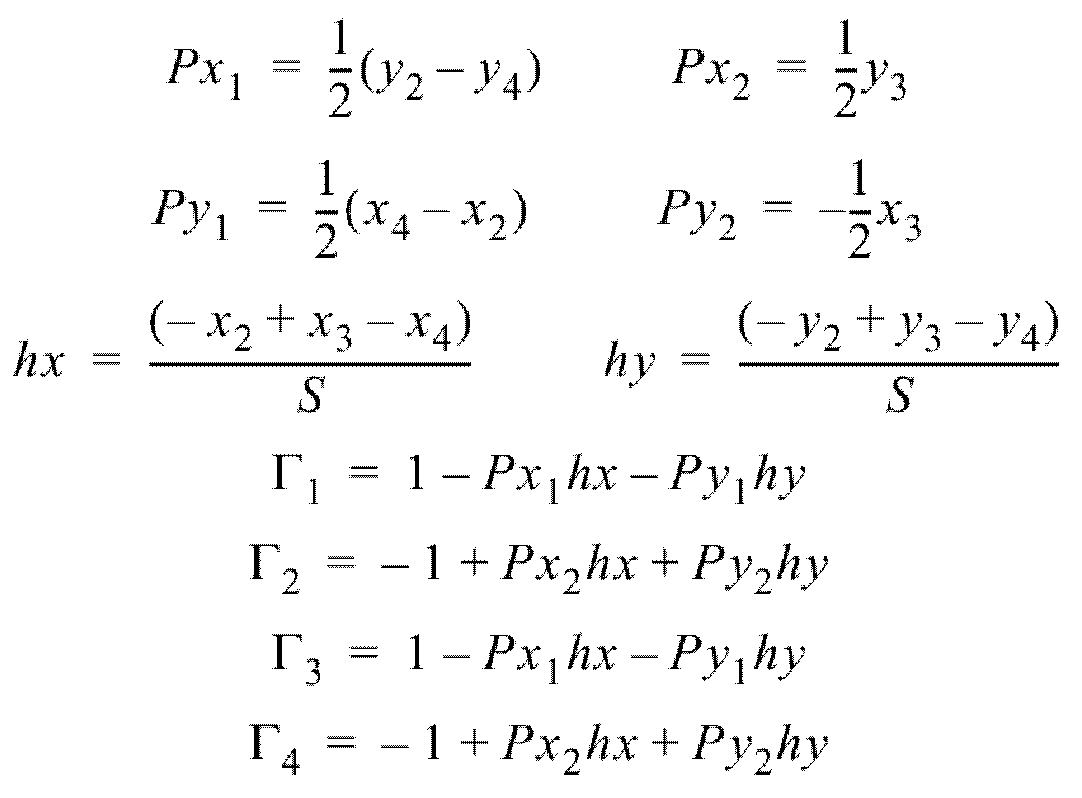
Decomposition on the hourglass base vectors gives ¹:(3)

\frac{\partial q_{i}^{α}}{\partial t} = Γ_{I}^{α} \cdot v_{i I}^{H o u r} = (v_{i I} - \frac{\partial v_{i I}}{\partial x_{j}} \cdot x_{j}) \cdot Γ_{I}^{α}

Where,

$\frac{\partial q_{i}^{α}}{\partial t}$: Hourglass modal velocities
$Γ_{I}^{α}$: Hourglass vectors, base

Remembering that

\frac{\partial v_{i}}{\partial x_{j}} = \frac{\partial Φ_{j}}{\partial x_{j}} \cdot v_{i J}

and factorizing Hourglass Modes, Equation 5 gives:(4)

\frac{\partial q_{i}^{α}}{\partial t} = v_{i I} \cdot (Γ_{I}^{α} - \frac{\partial Φ_{J}}{\partial x_{j}} x_{j} Γ_{J}^{α})

(5)

γ_{I}^{α} = Γ_{I}^{α} - \frac{\partial Φ_{J}}{\partial x_{j}} x_{j} Γ_{J}^{α}

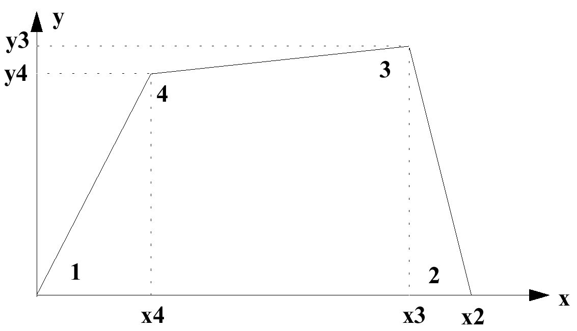
is the hourglass shape vector used in place of

Γ_{I}^{α}

in Hourglass Modes, Equation 2.

Elastoplastic Hourglass Forces

I_shell=3

The same formulation as elastic hourglass forces is used (Hourglass Elastic Stiffness Forces and Flanagan et al. ¹) but the forces are bounded with a maximum force depending on the current element mean yield stress. The hourglass forces are defined as:(6)

f_{i I}^{h g r} = f_{i}^{h g r} Γ_{I}

For in plane mode:(7)

f_{i}^{h g r} (t + Δ t) = f_{i}^{h g r} (t) + \frac{1}{8} h_{m} E t \frac{\partial q_{i}}{\partial t} Δ t

(8)

f_{i}^{h g r} (t + Δ t) = \min (f_{i}^{h g r} (t + Δ t), \frac{1}{2} h_{m} σ_{y} t \sqrt{A})

For out of plane mode:(9)

f_{i}^{h g r} (t + Δ t) = f_{i}^{h g r} (t) + \frac{1}{40} h_{f} E t^{3} \frac{\partial q_{i}}{\partial t} Δ t

(10)

f_{i}^{h g r} (t + Δ t) = \min (f_{i}^{h g r} (t + Δ t), \frac{1}{4} h_{f} σ_{y} t^{2})

Where,

$t$: Element thickness
$σ_{y}$: Yield stress
$A$: Element area

Physical Hourglass Forces

I_shell=22, 24

The hourglass forces are given by:(11)

f^{{int}^{h g r}} = \int_{Ω e} B^{H t} C B^{H} v d Ω^{e}

For in-plane membrane rate-of-deformation, with

Φ = ξ η

and

γ_{I}

defined in Bilinear Shape Functions, Equation 3:(12)

[{(B_{I}^{m})}^{H}] = [\begin{matrix} γ_{I} ϕ, x & 0 & 0 \\ 0 & γ_{I} ϕ, y & 0 \\ γ_{I} ϕ, y & γ_{I} ϕ, x & 0 \end{matrix}]

For bending:(13)

[{(B_{I}^{b})}^{H}] = [\begin{matrix} 0 & γ_{I} ϕ, x \\ - γ_{I} ϕ, y & 0 \\ - γ_{I} ϕ, x & γ_{I} ϕ, y \end{matrix}]

It is shown in ² that the non-constant part of the membrane strain rate does not vanish when a warped element undergoes a rigid body rotation. Thus, a modified matrix [

{(B_{I}^{m})}^{H}

] is chosen using

z_{γ} = γ_{I} z^{I}

as a measure of the warping:(14)

[{(B_{I}^{m})}^{H}] = [\begin{matrix} γ_{I} ϕ_{, x} & 0 & z_{γ} b_{x I} ϕ,_{x} \\ 0 & γ_{I} ϕ_{, y} & z_{γ} b_{y I} ϕ,_{y} \\ γ_{I} ϕ_{, y} & γ_{I} ϕ_{, x} & z_{γ} (b_{x I} ϕ,_{y} + b_{y I} ϕ,_{x}) \end{matrix}]

This matrix is different from the Belytschko-Leviathan ³ correction term added at rotational positions, which couples translations to curvatures as:(15)

[{(B_{I}^{m})}^{H}] = [\begin{matrix} γ_{I} ϕ_{, x} & 0 & 0 & 0 & - \frac{1}{4} z_{γ} ϕ_{, x} \\ 0 & γ_{I} ϕ_{, y} & 0 & \frac{1}{4} z_{γ} ϕ_{, y} & 0 \\ γ_{I} ϕ_{, y} & γ_{I} ϕ_{, x} & 0 & \frac{1}{4} z_{γ} ϕ_{, x} & - \frac{1}{4} z_{γ} ϕ_{, y} \end{matrix}]

This will lead to membrane locking (the membrane strain will not vanish under a constant bending loading). According to the general formulation, the coupling is presented in terms of bending and not in terms of membrane, yet the normal translation components in ( $B_{I}^{m}$ ) do not vanish for a warped element due to the tangent vectors $t_{i} (ξ, η)$ which differ from $t_{i} (0, 0)$ .

Fully Integrated Formulation

I_shell=12

The element is based on the Q4 $γ$ 24 shell element developed in ⁴ by Batoz and Dhatt. The element has 4 nodes with 5 local degrees-of-freedom per node. Its formulation is based on the Cartesian shell approach where the middle surface is curved. The shell surface is fully integrated with four Gauss points. Due to an in-plane reduced integration for shear, the element shear locking problems are avoided. The element without hourglass deformations is based on Mindlin-Reissner plate theory where the transversal shear deformation is taken into account in the expression of the internal energy. Consult the reference for more details.

Shell Membrane Damping

The shell membrane damping, dm, is only used for LAWS 25, 27, 19, 32 and 36. The Shell membrane damping factor is a factor on the numerical VISCOSITY and not a physical viscosity. Its effect is shown in the formula of the calculation of forces in a shell element:

d m = d m

read in D00 input (Shell membrane damping factor parameter) then:(16)

d m = \sqrt{2} \cdot d m_{D 00} \cdot ρ_{0} \cdot c \cdot \sqrt{A R E A}

Effect in the force vector (

F

) calculation:(17)

F_{1 n e w} = F_{1 o l d} + d m ({\dot{ε}}_{11} + \frac{{\dot{ε}}_{22}}{2})

(18)

F_{2 n e w} = F_{2 o l d} + d m ({\dot{ε}}_{22} + \frac{{\dot{ε}}_{11}}{2})

(19)

F_{3 n e w} = F_{3 o l d} + d m \frac{{\dot{ε}}_{12}}{3}

Where,

$ρ_{0}$: Density
$A R E A$: Area of the shell element surface
dt: Time step
$c$: Sound speed

In order to calibrate the dm value so that it represents the physical viscosity, one should obtain the same size for all shell elements (Cf. $A R E A$ factor), then scale the physical viscosity value to the element size.

¹ Flanagan D. and Belytschko T., “A Uniform Strain Hexahedron and Quadrilateral with Orthogonal Hourglass Control”, Int. Journal Num. Methods in Engineering, 17 679-706, 1981.

² Belytschko T., Lin J.L. and Tsay C.S., “Explicit algorithms for the nonlinear dynamics of shells”, Computer Methods in Applied Mechanics and Engineering, 42:225-251, 1984.

³ Belytschko T. and Leviathan I., “Physical stabilization of the 4-node shell element with one-point quadrature”, Computer Methods in Applied Mechanics and Engineering, 113:321-350, 1992.

⁴ Batoz J.L. and Dhatt G., “Modeling of Structures by finite element”, volume 3, Hermes, 1992.