Deviatoric Stress Calculation

With the stress being separated into deviatoric and pressure (hydrostatic) stress (Stresses in Solids), it is the deviatoric stress that is responsible for the plastic deformation of the material. The hydrostatic stress will either shrink or expand the volume uniformly, i.e. with proportional change in shape. The determination of the deviatoric stress tensor and whether the material will plastically deform requires a number of steps.

Perform an Elastic Calculation

The deviatoric stress is time integrated from the previous known value using the strain rate to compute an elastic trial stress:(1)

s_{i j}^{e l} (t + Δ t) = s_{i j} (t) + {\dot{s}}_{i j}^{r} Δ t + 2 G ({\dot{ε}}_{i j} - \frac{1}{3} {\dot{ε}}_{k k} δ_{i j}) Δ t

Where,

$G$: Shear modulus

This relationship is Hooke's Law, where the strain rate is multiplied by time to give strain.

Compute von Mises Equivalent Stress and Current Yield Stress

Depending on the type of material being modeled, the method by which yielding or failure is determined will vary. The following explanation relates to an elastoplastic material (LAW2).

The von Mises equivalent stress relates a three dimensional state of stress back to a simple case of uniaxial tension where material properties for yield and plasticity are well known and easily computed.

The von Mises stress, which is strain rate dependent, is calculated using the equation:(2)

σ_{v m}^{e} = \sqrt{\frac{3}{2} s_{i j}^{e l} s_{i j}^{e l}}

The flow stress is calculated from the previous plastic strain:(3)

σ_{y} (t) = a + b ε^{p^{n}} (t)

For material laws 3, 4, 10, 21, 22, 23 and 36, Equation 3 is modified according to the different modeling of the material curves.

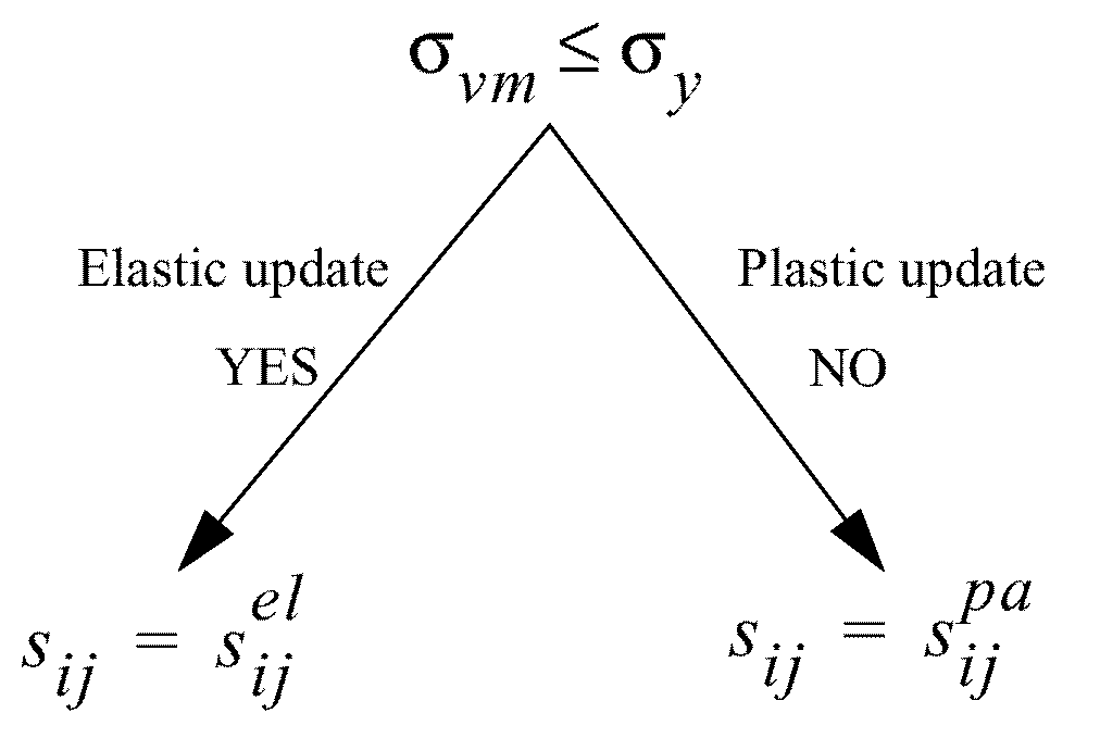
Plasticity Check

The state of the deformation must be checked.(4)

σ_{v m}^{e} - σ_{y} \leq 0

If this equation is satisfied, the state of stress is elastic. Otherwise, the flow stress has been exceeded and a plasticity rule must be used (Figure 1).

The plasticity algorithm used is due to Mendelson. ¹

Compute Hardening Parameter

The hardening parameter is defined as the slope of the strain-hardening part of the stress-strain curve:(5)

H = \frac{d σ_{y}}{d ε^{p}}

This is used to compute the plastic strain at time

t

:(6)

{\dot{ε}}^{p} Δ t = \frac{σ_{v m} - σ_{y}}{3 G + H}

This plastic strain is time integrated to determine the plastic strain at time

t + Δ t

:(7)

ε^{p} (t + Δ t) = ε^{p} (t) + {\dot{ε}}^{p} Δ t

The new flow stress is found using:(8)

σ_{y} (t + Δ t) = a + b ε^{p^{n}} (t + Δ t)

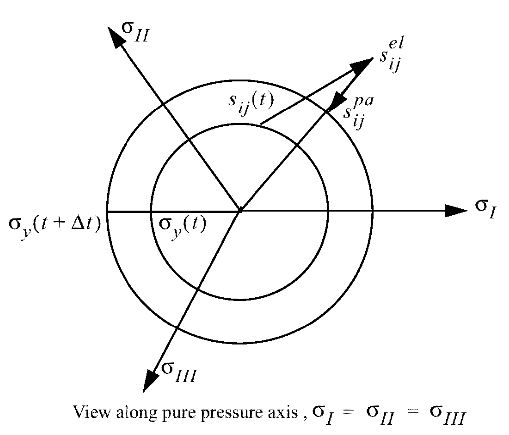
Radial Return

There are many possible methods for obtaining $s_{i j}^{p a}$ from the trial stress. The most popular method involves a simple projection to the nearest point on the flow surface, which results in the radial return method.

The radial return calculation is given in Equation 9. Figure 2 is a graphic representation of radial return.(9)

s_{i j}^{p a} = \frac{σ_{y}}{σ_{v m}} s_{i j}^{e l}