The Jaumann objective stress tensor derivative is the corrected true stress rate tensor without rotational
effects. The constitutive law is directly applied to the Jaumann stress rate tensor.
Deviatoric stresses and pressure (Stresses in Solids) are computed separately and
related by:(4)
Where,
Deviatoric stress tensor
Pressure or mean stress - defined as positive in compression
Substitution tensor or unit matrix
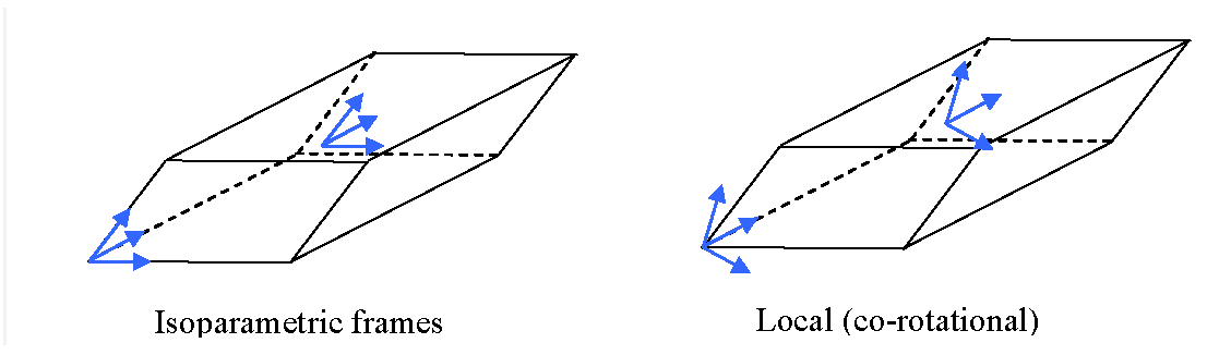
Co-rotational Formulation
A co-rotational formulation for bricks is a formulation where rigid body rotations are
directly computed from the element's node positions. Objective stress and strain tensors are
computed in the local (co-rotational) frame. Internal forces are computed in the local frame
and then rotated to the global system.
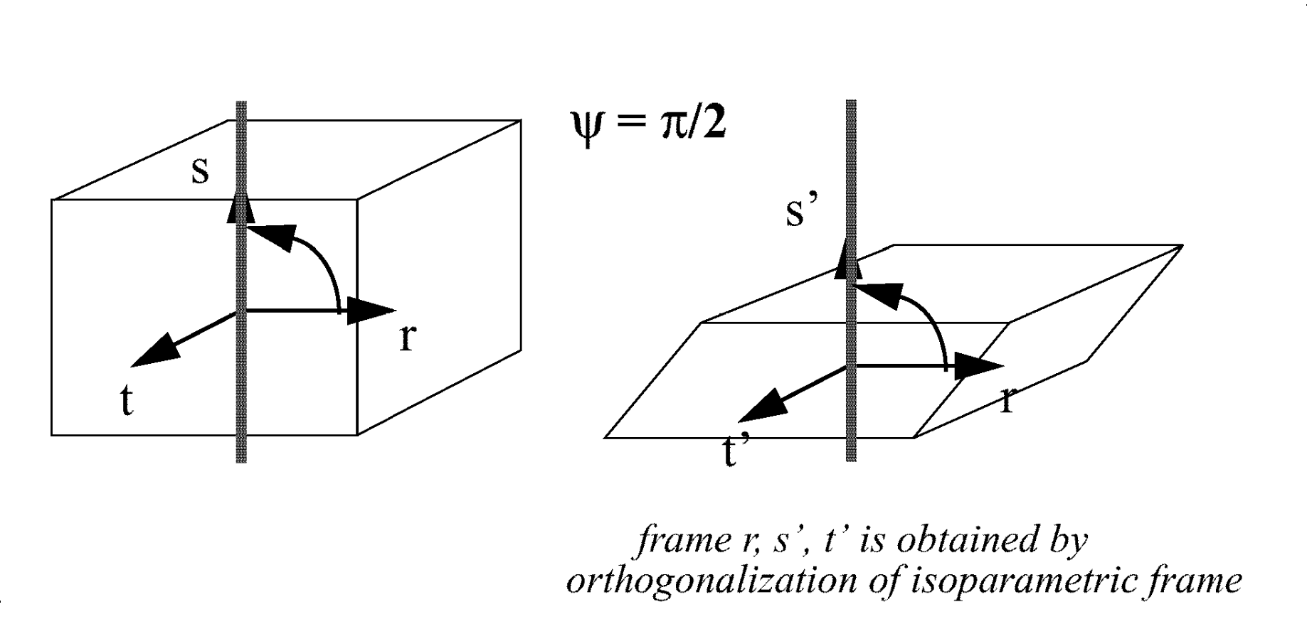
Jaumann objective stress tensor derivative expressed in the co-rotational frame
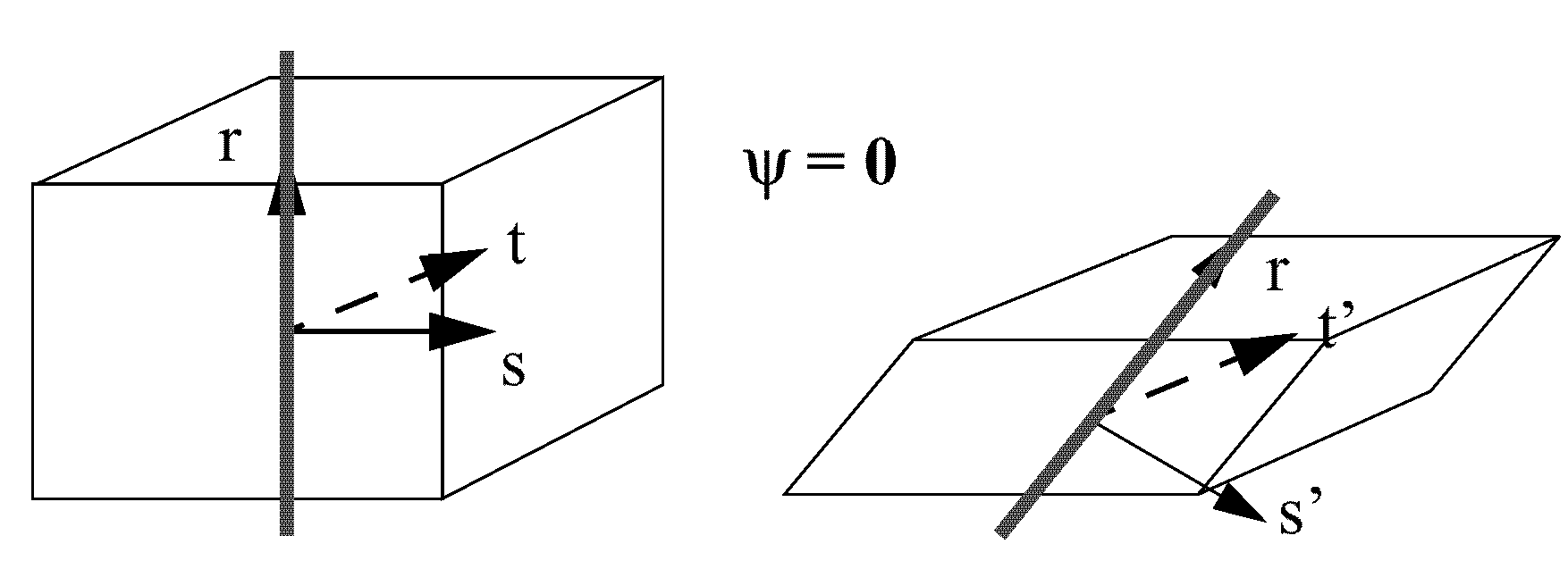
Figure 1 orthogonalization, when one of the
r, s, t directions is orthogonal to the two other directions. Figure 1.
When large rotations occur, this formulation is more accurate than the global formulation,
for which the stress rotation due to rigid body rotational velocity is computed in an
incremental way.
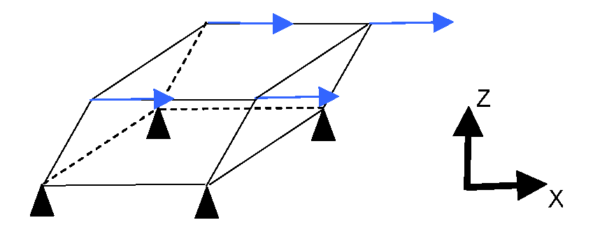
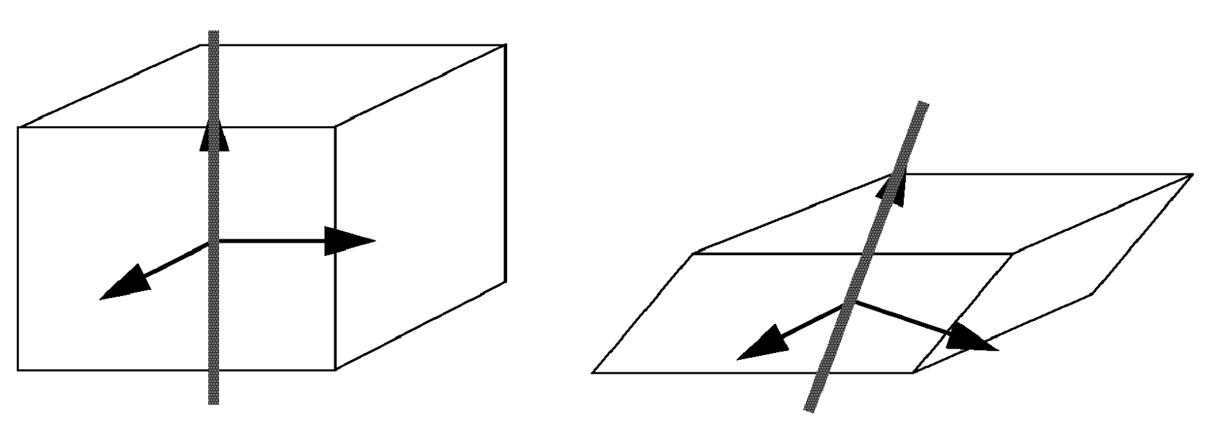
Co-rotational formulation avoids this kind of problem. Consider this test: Figure 2.
The increment of the rigid body rotation vector during time step is:(6)
So,
Where, equals the imposed velocity on the top of the brick divided by
the height of the brick (constant value).
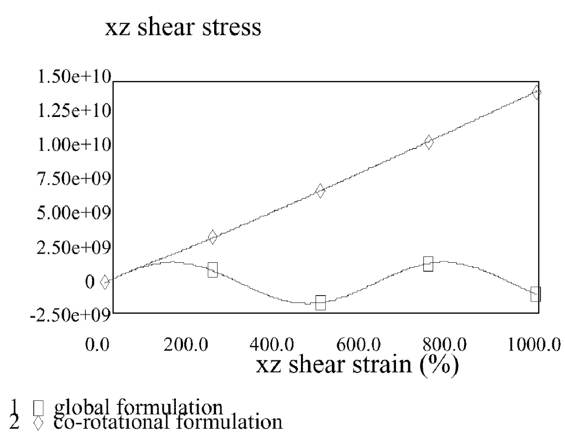
Due to first order approximation, the increment of stress due to the rigid body motion is:(7)
Increment of stress due to the rigid body motion:(8)
Increment of shear stress due to the rigid body motion:(9)
Increment of shear strain:(10)
Increment of stress due to strain:(11)
and increment of shear stress due to strain is:(12)
Where, is the shear modulus (material is
linear elastic).
So, shear stress is sinusoidal and is not strictly increasing. Figure 3.
So, it is recommended to use co-rotational formulation, especially for visco-elastic
materials such as foams, even if this formulation is more time consuming than the global
one.
Co-rotational Formulation
and Orthotropic Material
When orthotropic material and global formulation are
used, the fiber is attached to the first direction of the isoparametric frame and the fiber
rotates a different way depending on the element numbering. Figure 4. Figure 5.
On the other hand, when the co-rotational formulation is used, the orthotropic
frame keeps the same orientation with respect to the local (co-rotating) frame, and is
therefore also co-rotating. Figure 6.
1Wilkins M., “Calculation of elastic plastic flow” LLNL, University
of California UCRL-7322, 1981.