Boundary Conditions
Boundary conditions available for SimSolid Cloud.
Constraints
Structural constraints restrict or limit movement in specified regions of the model. For static analyses, models much be sufficiently constrained such that all rigid body motion is removed. Rigid body motion is defined as translation or rotational movement along or about the 3 primary (X, Y and Z) geometric axes.
In SimSolid Cloud, constraints (as well as loads) are applied to one or more part faces. To constrain a more local region split the face prior to importing the model.
Constraints are defined in the Analyses panel of the project tree. The type of constraints available in SimSolid Cloud include the following:
- Immovable support
- Enforces zero translational displacements in all directions. It is applied to one or more faces in the model.
- Slider support
- enforces zero displacement in directions normal to the surface direction. Displacements tangent to the surface are unconstrained. Sliding support can be used to define planes of symmetry.
- Hinge support
- Hinge supports allow a part to freely rotate about the center-line of a
cylindrical face but constrains movement in both the radial and axial
directions. Hinge supports can only be applied to full or partial
cylindrical faces. The cylindrical faces may be either concave or
convex.
Figure 1. 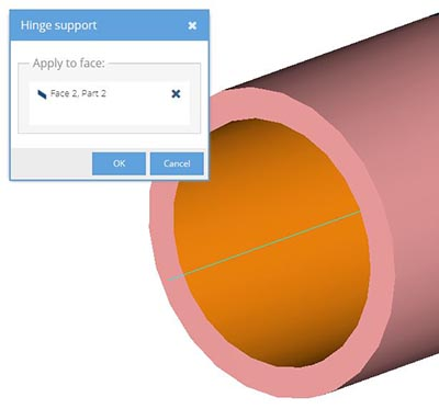
- Spring support
- Spring support allow general stiffness values to be applied to a support in the global X, Y and Z directions. Optionally, these may be defined in terms of volumetric foundation factors. Factors for several common materials such as concrete, wood, hard rubber, loose soil, compacted soil and railroad ballast are provided.
Loads
- Pressure
- A pressure load is defined as force per unit area and acts perpendicular to the part face. Pressure is assumed to be constant.
- Force/Displacement
- Both force and prescribed displacement are defined in a single dialog.
Force is defined as a load on the model. The specified value is
interpreted as a total force applied to all selected part faces. Loads
and prescribed displacement can be specified in global X, Y and Z
directions only.
Figure 2. Example of prescribed "0mm (fixed) displacement in X and a 100 N force in Y applied to single face 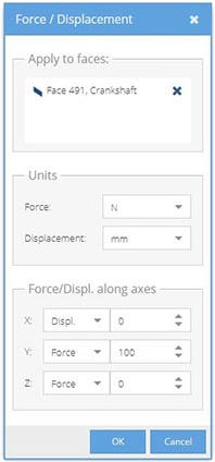
- Bearing load
- Bearing loads are nonuniform pressure loads applied to a region of any face of revolution (cylinder, cone, torus, and so on). They are defined by a direction and spread angle (10 – 180 degrees). The faces may be concave or convex. The selected point on the face indicates the initial load direction. You can apply bearing loads as a force in the radial or axial direction or as a moment on the selected face. The bearing load can be further adjusted by using the Load direction and Spread angle sliders. Since bearing loads only apply load to 1 side of the face, they are a more accurate representation of how a pin would transfer load in a hole.
- Gravity load
- Gravity is a body load uniformly distributed over the volumes of parts of an assembly. To apply a Gravity load, specify the X, Y and Z directional components of the gravity load in the dialog. When choosing a sign, note that a negative value opposes the coordinate direction. For example, if you want to simulate a downward gravitational force in the Y-direction, you enter “-1” in the Y field of the dialog. Optionally, a gravity amplification factor may be specified. This scales the gravity and can be used as a means to apply larger full body inertia forces. The default is a standard 1 G gravitational load. Only one gravity load can be applied per analysis. Gravity load acts on all unsuppressed parts of the assembly.
- Inertia loads
- An inertia load is a body load uniformly distributed over either a group
of parts or the entire assembly. In SimSolid Cloud, inertia loads may be either
Translational or Rotational.
- Translational - Translational inertia loads are in the global XYZ reference frame and are specified in terms of acceleration in a given direction. These loads are superposed with the gravity load if present.
- Rotational - Rotational inertia loads are applied with respect to an axis of rotation. Select a curved cylinder edge to locate the axis of rotation. If necessary, use the Flip axis button to change the way the axis points. Drag the ball and arrows to approximately position the origin point, then fine tune the text values on the dialog. Once positioned, simply specify the acceleration along the axis [α], angular velocity [ω] or angular acceleration [ε] as required and select OK to close the dialog.
Note: Inertia loads act in the opposite to direction specified. An acceleration in the +X direction causes a force in the -X direction. This is different to the gravity load which has a force in the direction specified. As a reference, common values for gravity at sea level are 9.81 m/s2 or 386.09 in/s2. - Inertia relief
- Inertia relief is applied to a structure in order to simulate deformations and stresses in cases where (1) the structure is unconstrained so it can move as a rigid body and (2) an active load is suddenly applied to the structure, so the structure starts moving with translational and rotational accelerations. Typical applications of inertial relief are an airplane in flight or a satellite in space. The solution to the problem of analysis of unconstrained structures is based on d’Alembert principal. The principal states that the structure will be in static equilibrium if the active loads are complimented by fictitious inertia loads evaluated through the structure accelerations. Therefore, in inertia relief analysis, fictitious inertia forces are calculated and distributed over the volume of the structure in such a way that they are in exact balance with the user applied forces. In SimSolid, when analyzing the inertial relief, there is no need to apply additional constraints which would eliminated rigid body motions of the structure. The user simply specifies the active loads and the rest is done automatically. Note that inertia relief cannot be combined with other inertia loads.
- Thermal load
- You can use results from a thermal analysis, or apply uniform temperature, to all parts or specific parts of the assembly to study the deformations and stresses due to temperature changes.
- Remote load
- Remote loads are used to apply distributed loads to select set of faces that are statically equivalent to a load applied to a single remote point. Static equivalency means that the applied traction exerts the same effect on the model as the force and/or moment applied to the selected point. The remote load is the only method for applying bending, twisting, or other moment loads to your model. To apply a remote load, first enter the remote point coordinates. Dragging the location on screen to roughly position it then use the text fields on the dialog to fine tune the values. Second, enter the force and/or moment directional components on the dialog.
- Distributed mass
- You can apply distributed mass across selected faces. Distributed mass can be applied using total mass or mass per area.
- Hydrostatic pressure
- Hydrostatic pressure is defined as a pressure exerted by a fluid at equilibrium at a given point within the fluid, due to the force of gravity. Hydrostatic pressure increases in proportion to depth measured from the surface because of the increasing weight of fluid exerting downward force from above.
- Temperature
- Specifies a constant fixed temperature on one or more groups of part faces.
- Heat Flux
- Specifies rate of heat energy transfer through a given surface per unit of time. Heat rate is given in Watts. Watts are defined as Joules per second. Heat flux is then Watts per unit of area. For example, in SI units, this is given as watt/m2.
- Volumetric Heat
- Specifies internal heat generation (heat sources) and internal heat absorption (heat sinks) in a given part volume. A positive volume heat value indicates a heat source, and a negative volume heat value indicates a heat sink. Volumetric heat is given as Watts per unit of volume. For example: W/m3.
- Convection
- Specifies the convection coefficient and ambient temperature on a given set of faces. The Ambient temperature defines the temperature of the bulk fluid, which is assumed to remain constant during the analysis. The convection coefficient defines the rate of heat transfer between the bulk fluid (liquid or gas, buoyant or moving) and a surface of your model. The convective coefficient is equal to the heat rate per unit area per unit temperature difference between the model surface and the bulk fluid. Units for convection coefficients are: W/(m2⋅K).
- Bolt and nut tightening
- Bolt and nut tightening loads are used to simulate pre-tensioning. Learn more here.