HV-3060: Transform and Average Stresses
Learn how to use various averaging methods for elemental stress and transform your results
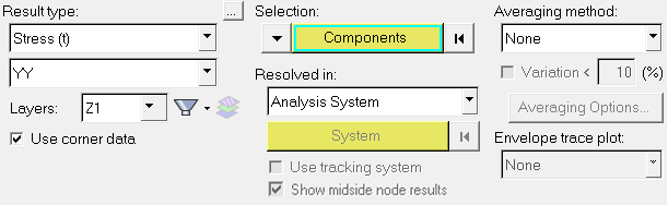
Figure 1.
Averaging of elemental results at a node refers to the average of all the element corner results passing through that node. If no corner results are available for an element, centroidal results will be used calculate the average. This option allows you to change the results from being element bound to being nodal bound. The various averaging options are Simple, Advanced, and Difference.
Contouring the Model Results
-
Click the Mask panel button
 on the Display
toolbar to enter the Mask panel.
on the Display
toolbar to enter the Mask panel.
-
Enter the following element IDs into the text box: 108, 16, 12,
107.
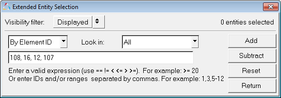 Figure 2.
 -
Select the Contour panel from the toolbar
 .
.
-
Click Apply.
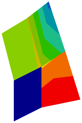 Figure 3.
 Observe the discontinuities in the contour around the node that is shared by all four elements.
Averaging the Elemental Stresses Using Various Averaging Methods
-
Click Apply.
 Figure 4. Note: The discontinuities around the node no longer exist, and you now are able to view the contour as bands.
Simple averaging means that tensor and vector components are extracted and the invariants are computed prior to averaging. In this example, the vonMises is computed at the corner of each element for the layer Z1 and then is averaged to the nodes.
-
Click OK.
The Resolved in system automatically changes to Global System (proj: x, y).
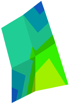 Figure 5.
 Advanced averaging means that tensor (or vector) results are transformed into a consistent system, and then each component is averaged separately to obtain an average tensor (or vector). In this example, the stress components xx, yy, zz, xy, yz, xz are computed at the corners and then averaged to the nodes. From this averaged value, the invariants (like vonMises) are computed. These results are more accurate with advanced averaging.
-
Activate the Feature angle averaging check box and leave
the Feature angle set to 50.
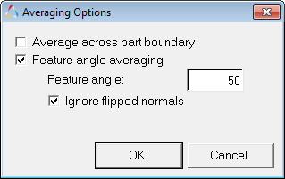 Figure 6.
 -
Click Apply to contour the model.
 Figure 7.
 -
Click Apply.
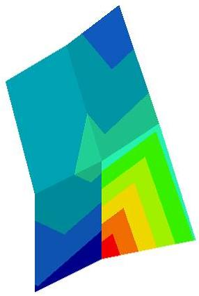 Figure 8.
 The variation is the relative difference at a node, with respect to all nodes in the selected components.
The formula is described as follows:
 Figure 9.
 -
Click Apply.
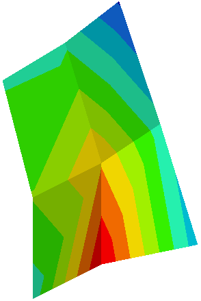 Figure 10.
 This option displays the difference between the maximum and minimum corner results at a node. For tensor/vector components, the corresponding components from each element corner are extracted and the difference is calculated. For invariants, the corresponding invariants are computed from each element corner and then the difference is calculated.