HV-3035: Post Process Complex Results
Learn how to post process complex results.
Complex results are supported in HyperView and can be
animated using the Modal Animation Mode, ![]() . After switching the
animation mode to modal, an additional option appears in the Contour panel which
allows the users to set the Complex filter.
. After switching the
animation mode to modal, an additional option appears in the Contour panel which
allows the users to set the Complex filter.
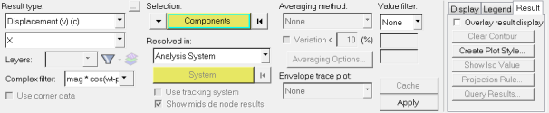 Figure 1.
 - mag*cos(ωt-phase)
- The response with varying angle or ωt (in degree).
- mag
- Magnitude (r) of the complex result.
- phase
- Phase
 of the complex number.
 - real
- Real part (x) of the complex number.
- imaginary
- Imaginary part (y) of the complex number.
Results that are complex are shown in the Result type list with a (c) appended to the result name. The other selections in the Contour panel are the same for complex results, as they are for non-complex results.
To view the contour of the complex response at a certain angle, use the Animation
Controls icon ![]() . Within the Animation
Controls panel, use the Current angle entry field to enter in the value for the
angle.
. Within the Animation
Controls panel, use the Current angle entry field to enter in the value for the
angle.
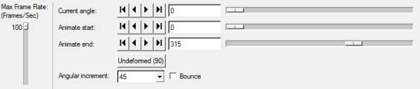 Figure 2.
 Also in the Animation Controls panel, the Angular Increment can also be set. This is
used when animating the model (see image above). To start the animation, click on
the Start/Pause Animation button ![]() .
.
The following exercise is an example of how post-processing complex results in HyperView is done. The model used in this exercise has four load cases. The first load case contains the static result. The second load case resets the model to an unloaded structure and is the base state used for load case 3 where the eigenfrequencies are extracted. In load case 4, the response of the mass element (element ID 999) on top of the clip due to a dynamic excitation (frequency dependent load) of the bearing in a node (node id 10000) is analyzed. The model is fixed in all six degrees of freedom at node 9999.
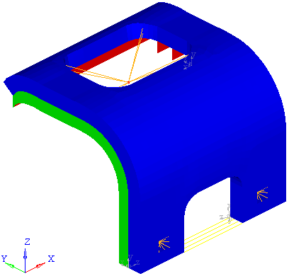 Figure 3.
 Import the Model into HyperView and Set the Animation Mode to Modal
-
Click the arrow next to the Page Window Layout icon
 on the Page Controls toolbar, and select the three
window layout
on the Page Controls toolbar, and select the three
window layout  .
.
- Go to the Load Model panel by selecting from the main menu.
- Load the model file Postprocessing_demo.inp and the results file Postprocessing_demo.odb, located in the animation folder.
- Verify that the window on the left is the active window (it will have a cyan box surrounding it).
- Click Apply to bring the model and results into HyperView.
-
Click on the downward pointing arrow next to the Animation Mode Menu icon
 and select
  Set Modal Animation Mode.
Set the Load Case to Load Case 4 and Contour the Model
-
From the Results Browser, use the Change load case drop-down menu to set the
load case to Step-4.
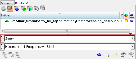 Figure 4. Note: The Change load case toolbar visibility can be toggled on/off using the Configure Browser option (located in the Results Browser context menu).
 -
Click the Contour panel button
 on the Result toolbar to enter the Contour panel.
-
Notice that the Complex filter field is activated. Click on the drop down and
select real to contour the model with the real component
of the velocity in the global z direction.
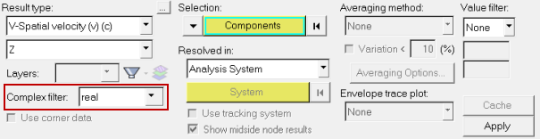 Figure 5.
 -
Click Apply.
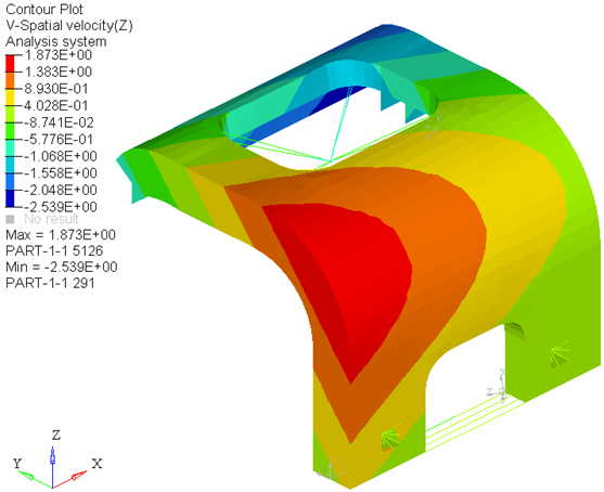 Figure 6.
Set the Animation Parameters and Animate the Model
-
Click on the Animation Controls button
 .
This panel allows users to set the Current angle of the animation and also the Angular Increment of the animation.
.
This panel allows users to set the Current angle of the animation and also the Angular Increment of the animation. -
Click the Start/Pause Animation button
 to start the animation.
-
Click the Start/Pause Animation button
 to stop/pause the animation.
Create a Measure of the Nodal Value at Node 999 and Plot the Values
-
Click the Measure panel button
 on the Annotation toolbar to enter the Measure panel.
-
Check the option for Live link.
The Live link option creates a link between the selections made on the measure panel and the curve. When a live measure item is deleted, a message is displayed prompting you to either keep or delete the curve.
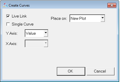 Figure 7.
 -
Click OK. This creates a curve in the second window
which has the phase angle in degrees on the x-axis and the measure value on the
y-axis.
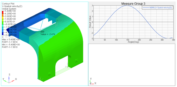 Figure 8. In HyperView, the formula used to create this plot is:
real*cos(wt)+imaginary*sin(wt)Not all post processors use this equation though. Another possible equation used by other post processors is the following:real*cos(wt)-imaginary*sin(wt)Notice the slight difference in the equations. Next you will plot this second equation on the same plot as the measure curve to illustrate that the difference between the two is simply a phase shift.
-
In the Curves toolbar, click the Define Curves panel
button
 to enter the Define Curves panel.
-
Click Apply.
Note: The curves are identical except for the phase shift.
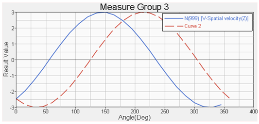 Figure 9.
Create a Complex Plot of the Time History Velocity Values
-
Set the plot type to Complex (see below).
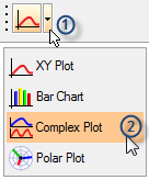 Figure 10.
 -
Select the Build Plots icon
 on the Curves toolbar.
-
For Data file, click the open file icon
 and select the file
Postprocessing_demo.odb.
and select the file
Postprocessing_demo.odb.
-
Make the following selections:
- For Y-Type, select V3-Spatial velocity (Time History)
- For Y-Request, select Node 999
- For Y-Component, select Value.
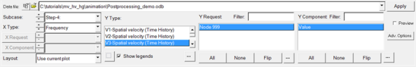 Figure 11.
 -
Click Apply.
This creates a complex plot with the Magnitude plotted on the bottom and the Phase plotted on the top.
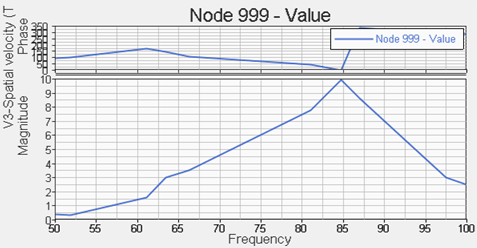 Figure 12.
 -
Right click in the third window and select Switch to
Real/Imaginary.
This updates the plot so that the Real component is plotted on the top and the Imaginary portion is plotted on the bottom.
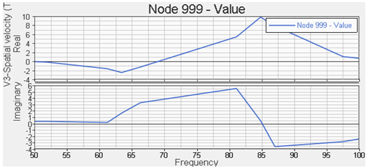 Figure 13.