HV-3055: Compare Scalar and Tensor Results from Abaqus
Learn how to contour scalar and tensor results using both shell and solid elements.
This exercise uses the model file Postprocessing_demo.inp and
the corresponding results file Postprocessing_demo.odb located in
the animation folder.
Set Up Two Windows and Import the File Postprocessing_demo.odb into Both Windows
-
Within HyperView, click on the drop-down menu next
to the Page Window Layout icon
 (on the PageControls toolbar), and select the following
Two Window Layout icon
(on the PageControls toolbar), and select the following
Two Window Layout icon  .
.
-
Click on the Reader Options… button.
The Reader Options dialog is displayed.
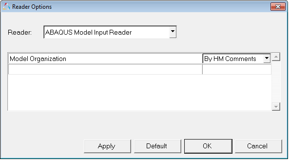 Figure 1.
 -
Click Apply to bring the model and result file into the
second window.
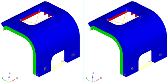 Figure 2.
Update the Display and Turn on the Display of Mesh Lines
-
From the Visualization toolbar, click on the Shaded Elements and
Mesh Lines icon
 to turn on the display of the mesh lines.
-
Repeat Step 1 in the other window so that both windows display the model with
mesh lines.
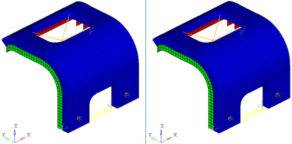 Figure 3.
 -
From the Results Browser, use the Change load case drop-down menu to set the
load case to Step-1.
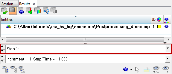 Figure 4. Note: The Change load case toolbar visibility can be toggled on/off using the Configure Browser option (located in the Results Browser context menu).
Apply a Contour of the Scalar Stress to the Shell Elements in the Left Window
-
Click the Contour panel button
 on the Result toolbar to enter the Contour panel.
-
Activate the Use corner data option check box.
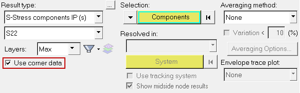 Figure 5.
 -
Click Apply to contour the model.
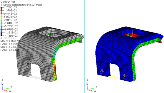 Figure 6.
Apply a Contour of the Tensor Stress to the Shell Elements in the Right Window
-
Activate the Use corner data option check box.
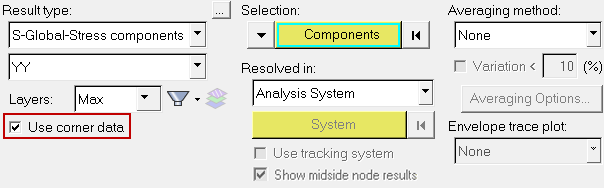 Figure 7.
 -
Click Apply to contour the model.
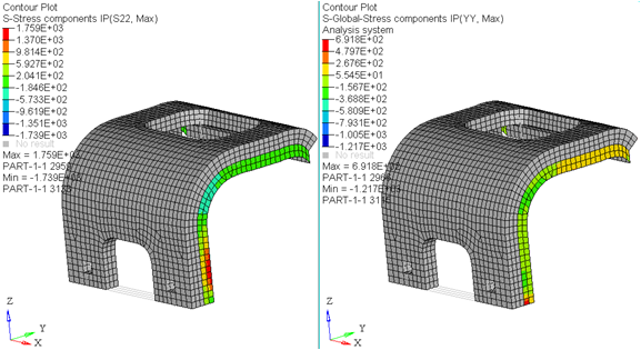 Figure 8. Note: The results are different between the scalar S22 and the tensor YY. One would expect that these two options would contour the same results (assuming that S22 corresponds to the Y direction). Remember that the scalar results are in a local coordinate system. For this analysis the local coordinate system has been defined as the following: the first axis is the global Y direction and the second axis is the global Z direction. Therefore, S22 actually corresponds to ZZ.
Update the Contour of the Tensor Stress in the Right Window
-
Click Apply to contour the model.
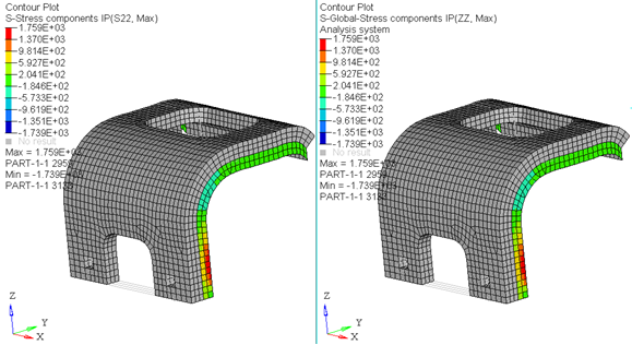 Figure 9. Note: Now the results match. Remember, shell elemental results are the in the local coordinate system for scalar results and in the global coordinate system for tensor results.
Apply a Contour of the Scalar Stress to the Solid Elements in the Left Window
-
Under Selection, reset the components selected by clicking on
 next to Components. In the graphics area, select the component displayed in
grey (this component contains only solid elements).
next to Components. In the graphics area, select the component displayed in
grey (this component contains only solid elements).
-
Click Apply to contour the solid elements.
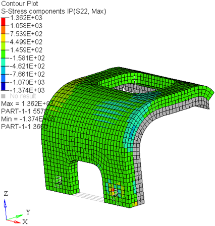 Figure 10.
Apply a Contour of the Tensor Stress to the Solid Elements in the Right Window
-
Under Selection, reset the components selected by clicking on
 next to Components. In the graphics area, select the
same grey component as was selected in Step 6/sub-Step 5 (above).
next to Components. In the graphics area, select the
same grey component as was selected in Step 6/sub-Step 5 (above).
-
Click Apply to contour the solid elements.
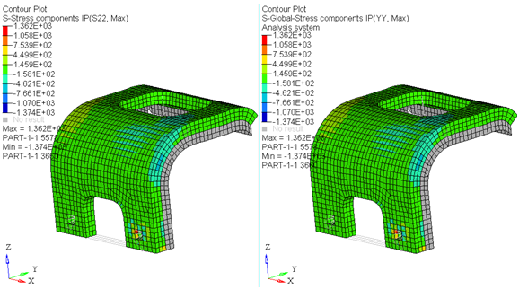 Figure 11. Note: In this example, the scalar results for S22 and the tensor results for YY match. This is because the elements that are contoured are solid elements. With solid elements, the scalar results are also in the global system.