This exercise uses the bullet_local.op2 model file located in
the animation folder.
In this tutorial, you will:
Create a stress contour on all components using the Results Browser
Create a contour on specific elements using stress results
Create an averaged stress contour and generate iso surfaces
Create a Plot Style to be used in the Results Browser
Contour vector and tensor results resolved in different coordinate
systems
Edit the legend
To access the Contour panel:
Click the Contour panel button on the Result toolbar.
OR
Select Results > Plot > Contour from the menu bar.
Figure 1.
The Contour panel allows you to contour a
model and graphically visualize the results. In the Contour panel you can view
vector, tensor, or scalar type results.
To access the Results Browser:
Select View > Browsers > HyperView > Results from the menu bar.
Figure 2.
Create a Stress Contour on all Components using the Results Browser
Load the bullet_local.op2 file, located in the animation
folder.
Open the Results Browser by selecting View > Browsers > HyperView > Results.
Expand the Results, Tensor, and Stress folders.
Figure 3.
All available stress values are listed under the Stress
folder.
Click on the icon next to vonMises.
Figure 4.
The contour is applied to the model in the graphics area.
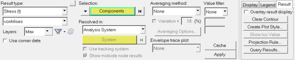
Alter the Contour Settings using the Contour Panel
The Contour panel allows you to contour a model and graphically visualize the
results. In the Contour panel you can view vector, tensor, or scalar type
results.
Click the Contour panel button on the Result toolbar to enter the Contour panel.
Figure 5.
Using the Contour panel, additional options can be changed and applied to the
contour.
Set Entity with Layers to Z1.
The options for Entity with Layers are:
Max
Displays the maximum values between layers Z1 and Z2.
Min
Displays the minimum values between layers Z1 and Z2.
Extreme
Displays the maximum absolute values among the layers for each
entity.
Z1/Z2
Displays the layers for thick shells. These will vary based on the
solver type.
Verify that Resolved in is set to Analysis System and that the Averaging method
is set to None.
Click Apply.
By default, the results are applied to all the model components displayed on
the screen.
You can also select individual components from the model.
Figure 6.
Create a Contour on Specific Elements using Stress
Results
Change the active input collector from Components to
Elements.
In the graphics area, pick a few elements on the model.
Click Apply.
Press the SHIFT key and the left mouse button, and drag the mouse in the
graphics area, to draw a window over a specific area of the model.
The contour is applied to the elements that were chosen using the quick
window mode.
This can also be done for other entity types.
Figure 7.
Under Selection, click on Elements and choose
All from the pop up selection window.
Note: If your solver supports corner data, activate the Use corner
data option to view corner results.
Create an Averaged Stress Contour and Generate Iso
Surfaces
Change the Averaging Method to Simple.
Click Apply.
Click Show Iso Value.
Figure 8.
The color bands reflect the band settings for the legend.
Click in the graphics area and press T on the keyboard.
This allows you to view the iso surface while seeing the model in transparent
mode.
Press T again to turn off transparency.
Click Clear Iso Value.
Click Create Plot Style.
Creating a plot style allows you to save the current settings in the Contour
panel so that they can be accessed later in the Results Browser.
In the Create/Update Contour Plot Style dialog, New plot
style text field, enter Simple vonMises and click
OK.
Figure 9.
In the Results Browser, expand the Plot Styles folder.
Note: Simple vonMises is now listed as a plot style.
Figure 10.
Click on Default Contour (under Plot Styles) to contour
the model with displacement results using the default contour plot style.
Observe the updates in the Contour panel.
Figure 11.
Click on Simple vonMises (under Plot Styles) to return
to the previous contour settings.
In the Results Browser, right click and select Clear Plot > Contour to remove the contour plot.
Contour Vector and Tensor Results Resolved in Different Coordinate Systems
For vector and tensor results, you can transform the results to a different
coordinate system.
Within the Contour panel select the following:
Set the Result type to Displacement (v).
Set the Data component to X.
Select the Analysis coordinate system.
Click Apply.
Set Resolved in to Global System (proj: none).
Click Apply.
Figure 12. Analysis SystemFigure 13. Global System
Clear the contour.
Change the following settings:
Set result type to Stress (t).
Set the data component to vonMises.
Under Resolved in select User System (proj: none).
Click Projection Rule, select Projection (use
projected axis as Sxx), and click
OK.
The current system changes to User System (proj: x, y).
Click on System and then click on By
ID.
Enter 2 to choose the second user defined system, and
click OK.
Figure 14.
Click Apply.
From the Results Browser, select Simple vonMises
(located under the Plot Styles folder) and observe the changes.
Edit the Legend
Click Edit Legend to open the Edit
Legend dialog.
Click on 4.514E+01 and change the value to
45.0.
The numbers will automatically interpolate and change in the preview
window.
Click Apply.
Observe the legend changes in the graphics screen.
 on the Result toolbar.
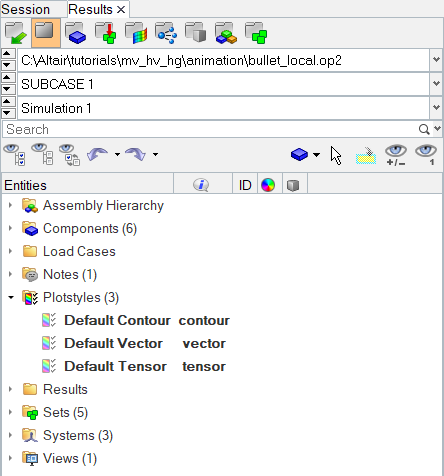
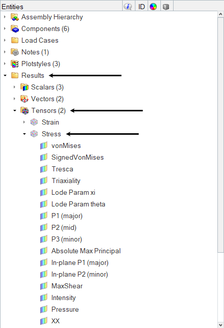 Figure 3. All available stress values are listed under the Stress folder.
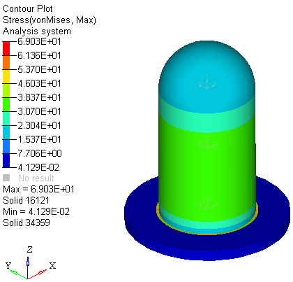 Figure 4. The contour is applied to the model in the graphics area.
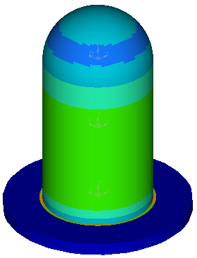 Figure 6.
 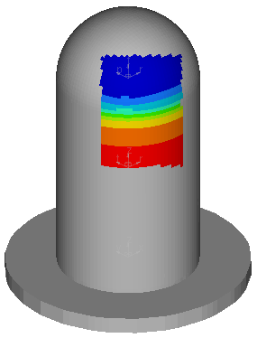 Figure 7.
 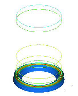 Figure 8. The color bands reflect the band settings for the legend.
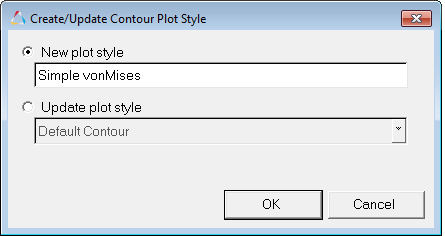 Figure 9.
 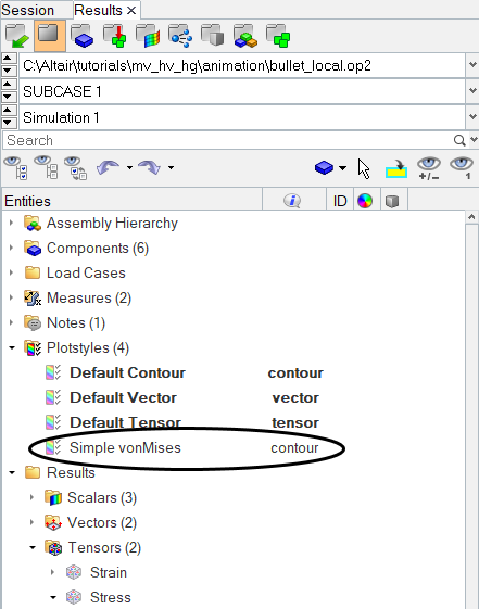 Figure 10.
 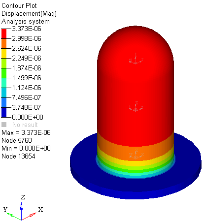 Figure 11.
 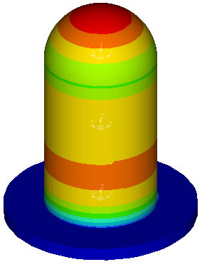 Figure 12. Analysis System
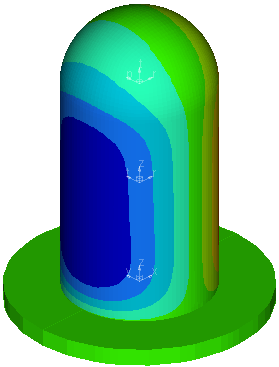 Figure 13. Global System
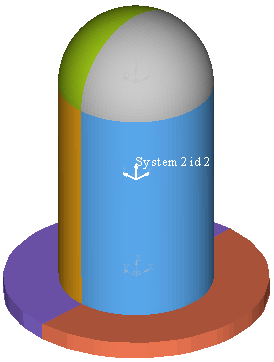 Figure 14.