Tabulated Piecewise Linear and Quadratic Elasto-plastic Laws (LAW36 and LAW60)

The elastic-plastic behavior of isotropic material is modeled with user-defined functions for work hardening curve.

The elastic portion of the material stress-strain curve is modeled using the elastic modulus, E, and Poisson's ratio, υ 
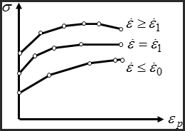
. The hardening behavior of the material is defined in function of plastic strain for a given strain rate (Figure 1). An arbitrary number of material plasticity curves can be defined for different strain rates. For a given strain rate, a linear interpolation of stress for plastic strain change, can be used. This is the case of LAW36 in Radioss. However, in LAW60 a quadratic interpolation of the functions allows to better simulate the strain rate effects on the behavior of material as it is developed in LAW60. For a given plastic strain, a linear interpolation of stress for strain rate change is used. Compared to Johnson-Cook model (LAW2), there is no maximum value for the stress. The curves are extrapolated if the plastic deformation is larger than the maximum plastic strain. The hardening model may be isotropic, kinematic or a combination of the two models as described in Cowper-Symonds Plasticity Model (LAW44). The material failure model is the same as in Zhao law.

For some kinds of steels the yield stress dependence to pressure has to be incorporated especially for massive structures. The yield stress variation is then given by:(1)
σ γ = σ γ 0 ( ε p ) × f ( p ) MathType@MTEF@5@5@+= feaagKart1ev2aaatCvAUfeBSjuyZL2yd9gzLbvyNv2CaerbwvMCKf MBHbqefqvATv2CG4uz3bIuV1wyUbqedmvETj2BSbqefm0B1jxALjhi ov2DaebbnrfifHhDYfgasaacH8srps0lbbf9q8WrFfeuY=Hhbbf9v8 qqaqFr0xc9pk0xbba9q8WqFfea0=yr0RYxir=Jbba9q8aq0=yq=He9 q8qqQ8frFve9Fve9Ff0dmeaacaGacmGadaWaaiqacaabaiaafaaake aacqaHdpWCdaWgaaWcbaGaeq4SdCgabeaakiabg2da9iabeo8aZnaa DaaaleaacqaHZoWzaeaacaaIWaaaaOGaaGPaVpaabmaabaGaeqyTdu 2aaSbaaSqaaiaadchaaeqaaaGccaGLOaGaayzkaaGaey41aqRaamOz amaabmaabaGaamiCaaGaayjkaiaawMcaaaaa@4D3E@
Where, p MathType@MTEF@5@5@+= feaagKart1ev2aaatCvAUfeBSjuyZL2yd9gzLbvyNv2CaerbwvMCKf MBHbqefqvATv2CG4uz3bIuV1wyUbqedmvETj2BSbqefm0B1jxALjhi ov2DaebbnrfifHhDYfgasaacH8srps0lbbf9q8WrFfeuY=Hhbbf9v8 qqaqFr0xc9pk0xbba9q8WqFfea0=yr0RYxir=Jbba9q8aq0=yq=He9 q8qqQ8frFve9Fve9Ff0dmeaacaGacmGadaWaaiqacaabaiaafaaake aacaWGWbaaaa@39CC@ is the pressure defined by Stresses in Solids, Equation 2. Drücker-Prager model described in Drücker-Prager (LAW10 and LAW21) gives a nonlinear function for f ( p ) . However, for steel type materials where the dependence to pressure is low, a simple linear function may be considered:(2)
σ y = σ y 0 ( ε p ) × C × p ( ε p ) MathType@MTEF@5@5@+= feaagKart1ev2aaatCvAUfeBSjuyZL2yd9gzLbvyNv2CaerbwvMCKf MBHbqefqvATv2CG4uz3bIuV1wyUbqedmvETj2BSbqefm0B1jxALjhi ov2DaebbnrfifHhDYfgasaacH8srps0lbbf9q8WrFfeuY=Hhbbf9v8 qqaqFr0xc9pk0xbba9q8WqFfea0=yr0RYxir=Jbba9q8aq0=yq=He9 q8qqQ8frFve9Fve9Ff0dmeaacaGacmGadaWaaiqacaabaiaafaaake aacqaHdpWCdaWgaaWcbaGaamyEaaqabaGccqGH9aqpcqaHdpWCdaqh aaWcbaGaamyEaaqaaiaaicdaaaGccaaMc8+aaeWaaeaacqaH1oqzda WgaaWcbaGaamiCaaqabaaakiaawIcacaGLPaaacqGHxdaTcaWGdbGa ey41aqRaamiCamaabmaabaGaeqyTdu2aaSbaaSqaaiaadchaaeqaaa GccaGLOaGaayzkaaaaaa@50B2@
Where,
C MathType@MTEF@5@5@+= feaagKart1ev2aaatCvAUfeBSjuyZL2yd9gzLbvyNv2CaerbuLwBLn hiov2DGi1BTfMBaeXatLxBI9gBaerbd9wDYLwzYbItLDharqqtubsr 4rNCHbGeaGqiVu0Je9sqqrpepC0xbbL8F4rqqrFfpeea0xe9Lq=Jc9 vqaqpepm0xbba9pwe9Q8fs0=yqaqpepae9pg0FirpepeKkFr0xfr=x fr=xb9adbaqaaeGaciGaaiaabeqaamaabaabaaGcbiqaaq1acaWGPb aaaa@373E@
User-defined constant
p MathType@MTEF@5@5@+= feaagKart1ev2aaatCvAUfeBSjuyZL2yd9gzLbvyNv2CaerbuLwBLn hiov2DGi1BTfMBaeXatLxBI9gBaerbd9wDYLwzYbItLDharqqtubsr 4rNCHbGeaGqiVu0Je9sqqrpepC0xbbL8F4rqqrFfpeea0xe9Lq=Jc9 vqaqpepm0xbba9pwe9Q8fs0=yqaqpepae9pg0FirpepeKkFr0xfr=x fr=xb9adbaqaaeGaciGaaiaabeqaamaabaabaaGcbiqaaq1acaWGPb aaaa@373E@
Computed pressure for a given deformed configuration
Chard in /MAT/LAW36 is same like in /MAT/LAW44. For more detail on Chard, see Cowper-Symonds Plasticity Model (LAW44).


Figure 1. Piecewise Linear Stress-Strain Curves
The principal strain rate is used for the strain rate definition:(3)
d ε d t = 1 2 ( d ε x d t + d ε y d t + ( d ε x d t d ε y d t ) 2 + ( d γ x y d t ) 2 ) MathType@MTEF@5@5@+= feaagKart1ev2aaatCvAUfeBSjuyZL2yd9gzLbvyNv2CaerbwvMCKf MBHbqefqvATv2CG4uz3bIuV1wyUbqedmvETj2BSbqefm0B1jxALjhi ov2DaebbnrfifHhDYfgasaacH8srps0lbbf9q8WrFfeuY=Hhbbf9v8 qqaqFr0xc9pk0xbba9q8WqFfea0=yr0RYxir=Jbba9q8aq0=yq=He9 q8qqQ8frFve9Fve9Ff0dmeaacaGacmGadaWaaiqacaabaiaafaaake aadaWcaaqaaiaadsgacqaH1oqzaeaacaWGKbGaamiDaaaacqGH9aqp daWcaaqaaiaaigdaaeaacaaIYaaaamaabmaabaWaaSaaaeaacaWGKb GaeqyTdu2aaSbaaSqaaiaadIhaaeqaaaGcbaGaamizaiaadshaaaGa ey4kaSYaaSaaaeaacaWGKbGaeqyTdu2aaSbaaSqaaiaadMhaaeqaaa GcbaGaamizaiaadshaaaGaey4kaSYaaOaaaeaadaqadaqaamaalaaa baGaamizaiabew7aLnaaBaaaleaacaWG4baabeaaaOqaaiaadsgaca WG0baaaiabgkHiTmaalaaabaGaamizaiabew7aLnaaBaaaleaacaWG 5baabeaaaOqaaiaadsgacaWG0baaaaGaayjkaiaawMcaamaaCaaale qabaGaaGOmaaaakiabgUcaRmaabmaabaWaaSaaaeaacaWGKbGaeq4S dC2aaSbaaSqaaiaadIhacaWG5baabeaaaOqaaiaadsgacaWG0baaaa GaayjkaiaawMcaamaaCaaaleqabaGaaGOmaaaaaeqaaaGccaGLOaGa ayzkaaaaaa@6793@

For strain rate filtering, refer to Strain Rate Filtering.