Cowper-Symonds Plasticity Model (LAW44)

This law models an elasto-plastic material with:

• Isotropic and kinematic hardening
• Tensile rupture criteria

The damage is neglected in the model. The work hardening model is similar to the Johnson-Cook model (LAW2) without temperature effect where the only difference is in the strain rate dependent formulation. The equation that describes the stress during plastic deformation is:(1)

$$\sigma =\left(a+b{\epsilon }_p{}^n\right)\left(1+{\left(\frac{\dot{\epsilon }}{c}\right)}^{\raisebox{1ex}{$1$}\!\left/ \!\raisebox{-1ex}{$p$}\right.}\right)$$

Where,

$\sigma$

Flow stress (Elastic + Plastic Components)

${\epsilon }_p$

Plastic strain (True strain)

$a$

Yield stress

$b$

Hardening modulus

$n$

Hardening exponent

$c$

Strain rate coefficient

$\dot{\epsilon }$

Strain rate

$\raisebox{1ex}{$1$}\!\left/ \!\raisebox{-1ex}{$p$}\right.$

Strain rate exponent

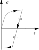
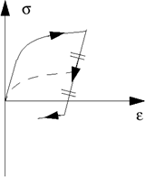
In isotropic hardening model, the yield surface inflates without moving in the space of principle stresses. The evolution of the equivalent stress defines the size of the yield surface, as a function of the equivalent plastic strain. The model can be represented in one dimensional case as shown in Table 1. When the loading direction is changed, the material is unloaded and the strain reduces. A new hardening starts when the absolute value of the stress reaches the last maximum value (Table 1 (a)).