Viscous Materials

General case of viscous materials represents a time-dependent inelastic behavior.

However, special attention is paid to the viscoelastic materials such as polymers exhibiting a rate- and time-dependent behavior. The viscoelasticity can be represented by a recoverable instantaneous elastic deformation and a non-recoverable viscous part occurring over the time. The characteristic feature of viscoelastic material is its fading memory. In a perfectly elastic material, the deformation is proportional to the applied load. In a perfectly viscous material, the rate of change of the deformation over time is proportional to the load. When an instantaneous constant tensile stress

σ_{0}

is applied to a viscoelastic material, a slow continuous deformation of the material is observed. When the resulting time dependent strain

ε (t)

, is measured, the tensile creep compliance is defined as:(1)

D (t) = \frac{ε (t)}{σ_{0}}

The creep behavior is mainly composed of three phases:

Primary creep with fast decrease in creep strain rate
Secondary creep with slow decrease in creep strain rate
Tertiary creep with fast increase in creep strain rate.

The creep strain rate is the slope of creep strain to time curve.

Another kind of loading concerns viscoelastic materials subjected to a constant tensile strain,

ε_{0}

. In this case, the stress,

σ (t)

which is called stress relaxation, gradually decreases. The tensile relaxation modulus is then defined as:(2)

E (t) = \frac{σ (t)}{ε_{0}}

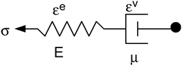
Because viscoelastic response is a combination of elastic and viscous responses, the creep compliance and the relaxation modulus are often modeled by combinations of springs and dashpots. A simple schematic model of viscoelastic material is given by the Maxwell model shown in Figure 1. The model is composed of an elastic spring with the stiffness

E

and a dashpot assigned a viscosity

μ

. It is assumed that the total strain is the sum of the elastic and viscous strains:(3)

ε = ε^{e} + ε^{v}

The time derivation of the last expression gives the expression of the total strain rate:(4)

\dot{ε} = {\dot{ε}}^{e} + {\dot{ε}}^{v}

As the dashpot and the spring are in series, the stress is the same in the two parts:(5)

σ^{e} = σ^{v} = σ

The constitutive relations for linear spring and dashpot are written as:(6)

$σ = E ε^{e}$ then $\dot{σ} = E {\dot{ε}}^{e}$

(7)

σ = μ {\dot{ε}}^{v}

Combining Equation 4, Equation 6 and Equation 7, an ordinary differential equation for stress is obtained:(8)

$\dot{σ} = E (\dot{ε} - \frac{σ}{μ})$ or $\dot{σ} = E \dot{ε} - \frac{σ}{τ}$

Where,

τ = \frac{μ}{E}

is the relaxation time. A solution to the differential equation is given by the convolution integral:(9)

σ (t) = \int_{- \infty}^{t} E e^{\frac{- (t - t')}{τ}} \frac{d ε (t')}{d t'} d t' = \int_{- \infty}^{t} R (t - t') \frac{d ε (t')}{d t'} d t'

Where,

R (t)

is the relaxation modulus. The last equation is valid for the special case of Maxwell one-dimensional model. It can be extended to the multi-axial case by:(10)

σ (t) = \int_{- \infty}^{t} C_{i j k l} (t - t') \frac{d ε (t')}{d t'} d t'

Where, $C_{i j k l}$ are the relaxation moduli. The Maxwell model represents reasonably the material relaxation. But it is only accurate for secondary creep as the viscous strains after unloading are not taken into account.

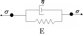
Another simple schematic model for viscoelastic materials is given by Kelvin-Voigt solid. The model is represented by a simple spring-dashpot system working in parallel as shown in Figure 2.

The mathematical relation of Kelvin-Voigt solid is written as:(11)

σ = E ε + η \dot{ε}

When $η = 0$ (no dashpot), the system is a linearly elastic system. When $E$ =0 (no spring), the material behavior is expressed by Newton's equation for viscous fluids. In the above relation, a one-dimensional model is considered. For multiaxial situations, the equations can be generalized and rewritten in tensor form.

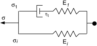
The Maxwell and Kelvin-Voigt models are appropriate for ideal stress relaxation and creep behaviors. They are not adequate for most of physical materials. A generalization of these laws can be obtained by adding other springs to the initial models as shown in Figure 3 and Figure 4. The equations related to the generalized Maxwell model are given as:(12)

σ = σ_{i} = σ_{1}

(13)

ε = \frac{σ_{i}}{E_{i}}

(14)

\dot{ε} = \frac{{\dot{σ}}_{1}}{E_{1}} + \frac{σ_{1}}{η_{1}}

The mathematical relations which hold the generalized Kelvin-Voigt model are: (15)

ε = ε^{e} + ε^{k}

$σ = σ^{e} + σ^{k}$

$ε^{e} = \frac{σ}{E}$ ; $ε^{k} = \frac{σ^{V}}{E_{t}}$ ; ${\dot{ε}}^{k} = \frac{σ^{V}}{η}$

The combination of these equations enables to obtain the expression of stress and strain rates: (16)

\dot{ε} = {\dot{ε}}^{e} + {\dot{ε}}^{k} = \frac{\dot{σ}}{E} + {\dot{ε}}^{k}

(17)

σ = η {\dot{ε}}^{k} + E_{t} ε^{k}

(18)

\dot{σ} = E \dot{ε} - \frac{(E - E_{t}) σ}{η} + \frac{E E_{t} ε}{η}

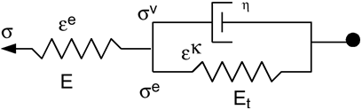
The models described above concern the viscoelastic materials. The plasticity can be introduced in the models by using a plastic spring. The plastic element is inactive when the stress is less than the yield value. The modified model is able to reproduce creep and plasticity behaviors. The viscoplasticity law (LAW33) in Radioss will enable to implement very general constitutive laws useful for a large range of applications as low density closed cells polyurethane foam, honeycomb, impactors and impact limiters.

The behavior of viscoelastic materials can be generalized to three dimensions by separating the stress and strain tensors into deviatoric and pressure components:(19)

s_{i j} = \int_{0}^{t} 2 Ψ (t - τ) \frac{\partial e_{i j}}{\partial τ} d τ

(20)

σ_{k k} (t) = \int_{0}^{t} 3 K (t - τ) \frac{\partial ε_{k k}}{\partial τ} d τ

Where, $s_{i j}$ and $e_{i j}$ are the stress and strain deviators. $ε_{k k}$ , $Ψ (t)$ and $K (t)$ are respectively the dilatation and the shear and bulk relaxation moduli.