Failure Models

In addition to the possibility to define user's material failure models, Radioss integrates several failure models. These models use generally a global notion of cumulative damage to compute failure. They are mostly independent to constitutive law and the hardening model and can be linked to several available material laws. A compatibility table is given in the Radioss Reference Guide. Table 1 provides a brief description of available models.
Table 1. Failure Model Description
Failure Model Type Description
BIQUAD Strain failure model Direct input on effective plastic strain to failure
CHANG Chang-Chang model Failure criteria for composites
CONNECT Failure Normal and Tangential failure model
EMC Extended Mohr Coulomb failure model Failure dependent on effective plastic strain
ENERGY Energy isotrop Specific energy
FABRIC Traction Strain failure
FLD Forming limit diagram Introduction of the experimental failure data in the simulation
HASHIN 3 4 Composite model Hashin model
HC_DSSE Extended Mohr Coulomb failure model Strain based Ductile Failure Model: Hosford-Coulomb with Domain of Shell-to-Solid Equivalence
JOHNSON Ductile failure model Cumulative damage law based on the plastic strain accumulation
LAD_DAMA Composite delamination Ladeveze delamination model
NXT NXT failure criteria Similar to FLD, but based on stresses
PUCK Composite model Puck model
SNCONNECT Failure Failure criteria for plastic strain
SPALLING Ductile + Spalling Johnson-Cook failure model with Spalling effect
TAB1 Strain failure model Based on damage accumulation using user-defined functions
TBUTCHER Failure due to fatigue Fracture appears when time integration of a stress expression becomes true
TENSSTRAIN Traction Strain failure
WIERZBICKI Ductile material 3D failure model for solid and shells
WILKINS Ductile Failure model Cumulative damage law

Johnson-Cook Failure Model

High-rate tests in both compression and tension using the Hopkinson bar generally demonstrate the stress-strain response is highly isotropic for a large scale of metallic materials. The Johnson-Cook model is very popular as it includes a simple form of the constitutive equations. In addition, it also has a cumulative damage law that can be accesses failure:(1)
D = Δ ε ε f MathType@MTEF@5@5@+= feaagKart1ev2aqatCvAUfeBSjuyZL2yd9gzLbvyNv2CaerbuLwBLn hiov2DGi1BTfMBaeXatLxBI9gBaerbd9wDYLwzYbItLDharqqtubsr 4rNCHbGeaGqiVu0Je9sqqrpepC0xbbL8F4rqqrFfpeea0xe9Lq=Jc9 vqaqpepm0xbba9pwe9Q8fs0=yqaqpepae9pg0FirpepeKkFr0xfr=x fr=xb9adbaqaaeGaciGaaiaabeqaamaabaabaaGcbaGaamiraiabg2 da9maaqaeabaWaaSaaaeaacaqGuoGaeqyTdugabaGaeqyTdu2aaSba aSqaaiaadAgaaeqaaaaaaeqabeqdcqGHris5aaaa@3F5E@
with:(2)
ε f = [ D 1 + D 2 exp ( D 3 σ * ) ] [ 1 + D 4 ln ( ε ˙ ε ˙ 0 ) ] [ 1 + D 5 T * ]

Where Δ ε is the increment of plastic strain during a loading increment, σ * = σ m σ V M the normalized mean stress and the parameters D i the material constants. Failure is assumed to occur when D MathType@MTEF@5@5@+= feaagKart1ev2aqatCvAUfeBSjuyZL2yd9gzLbvyNv2CaerbuLwBLn hiov2DGi1BTfMBaeXatLxBI9gBaerbd9wDYLwzYbItLDharqqtubsr 4rNCHbGeaGqiVu0Je9sqqrpepC0xbbL8F4rqqrFfpeea0xe9Lq=Jc9 vqaqpepm0xbba9pwe9Q8fs0=yqaqpepae9pg0FirpepeKkFr0xfr=x fr=xb9adbaqaaeGaciGaaiaabeqaamaabaabaaGcbaGaamiraaaa@36C0@ =1.

Wilkins Failure Criteria

An early continuum model for void nucleation is presented in 1. The model proposes that the decohesion (failure) stress σ c is a critical combination of the hydrostatic stress σ m and the equivalent von Mises stress σ V M :(3)
σ c = σ m + σ V M
In a similar approach, a failure criteria based on a cumulative equivalent plastic strain was proposed by Wilkins. Two weight functions are introduced to control the combination of damage due to the hydrostatic and deviatoric loading components. The failure is assumed when the cumulative reaches a critical value D c . The cumulative damage is obtained by:(4)
D c = W 1 W 2 d ε ¯ p i = 1 n W 1 W 2 Δ ε ¯ p i MathType@MTEF@5@5@+= feaagKart1ev2aqatCvAUfeBSjuyZL2yd9gzLbvyNv2CaerbuLwBLn hiov2DGi1BTfMBaeXatLxBI9gBaerbd9wDYLwzYbItLDharqqtubsr 4rNCHbGeaGqiVu0Je9sqqrpepC0xbbL8F4rqqrFfpeea0xe9Lq=Jc9 vqaqpepm0xbba9pwe9Q8fs0=yqaqpepae9pg0FirpepeKkFr0xfr=x fr=xb9adbaqaaeGaciGaaiaabeqaamaabaabaaGcbaGaamiramaaBa aaleaacaWGJbaabeaakiabg2da9maapeaabaGaam4vamaaBaaaleaa caaIXaaabeaakiaadEfadaWgaaWcbaGaaGOmaaqabaGccaaMc8Uaam izaiqbew7aLzaaraWaaSbaaSqaaiaadchaaeqaaaqabeqaniabgUIi YdGccqGHijYUdaaeWbqaaiaadEfadaWgaaWcbaGaaGymaaqabaGcca WGxbWaaSbaaSqaaiaaikdaaeqaaOGaaGPaVlaabs5acuaH1oqzgaqe amaaDaaaleaacaWGWbaabaGaamyAaaaaaeaacaWGPbGaeyypa0JaaG ymaaqaaiaad6gaa0GaeyyeIuoaaaa@5566@
Where,
W 1 = ( 1 1 + a P ) α
P = 1 3 j = 1 3 σ j j
W 2 = ( 2 A ) β
A = max ( s 2 s 3 , s 2 s 1 )
s 1 s 2 s 3
Where,
Δ ε ¯ p
An increment of the equivalent plastic strain
W 1 MathType@MTEF@5@5@+= feaagKart1ev2aqatCvAUfeBSjuyZL2yd9gzLbvyNv2CaerbuLwBLn hiov2DGi1BTfMBaeXatLxBI9gBaerbd9wDYLwzYbItLDharqqtubsr 4rNCHbGeaGqiVu0Je9sqqrpepC0xbbL8F4rqqrFfpeea0xe9Lq=Jc9 vqaqpepm0xbba9pwe9Q8fs0=yqaqpepae9pg0FirpepeKkFr0xfr=x fr=xb9adbaqaaeGaciGaaiaabeqaamaabaabaaGcbaGaam4vamaaBa aaleaacaaIXaaabeaaaaa@37BA@
Hydrostatic pressure weighting factor
W 2 MathType@MTEF@5@5@+= feaagKart1ev2aqatCvAUfeBSjuyZL2yd9gzLbvyNv2CaerbuLwBLn hiov2DGi1BTfMBaeXatLxBI9gBaerbd9wDYLwzYbItLDharqqtubsr 4rNCHbGeaGqiVu0Je9sqqrpepC0xbbL8F4rqqrFfpeea0xe9Lq=Jc9 vqaqpepm0xbba9pwe9Q8fs0=yqaqpepae9pg0FirpepeKkFr0xfr=x fr=xb9adbaqaaeGaciGaaiaabeqaamaabaabaaGcbaGaam4vamaaBa aaleaacaaIXaaabeaaaaa@37BA@
Deviatoric weighting factor
s i MathType@MTEF@5@5@+= feaagKart1ev2aqatCvAUfeBSjuyZL2yd9gzLbvyNv2CaerbuLwBLn hiov2DGi1BTfMBaeXatLxBI9gBaerbd9wDYLwzYbItLDharqqtubsr 4rNCHbGeaGqiVu0Je9sqqrpepC0xbbL8F4rqqrFfpeea0xe9Lq=Jc9 vqaqpepm0xbba9pwe9Q8fs0=yqaqpepae9pg0FirpepeKkFr0xfr=x fr=xb9adbaqaaeGaciGaaiaabeqaamaabaabaaGcbaGaam4CamaaBa aaleaacaaIXaaabeaaaaa@37D6@
Deviatoric principal stresses
a, α and β
The material constants

Tuler-Butcher Failure Criteria

A solid may break owning to fatigue due to Tuler-Butcher criteria: 2(5)
D = 0 t max ( 0 , ( σ σ r ) λ ) d t
Where,
σ r
Fracture stress
σ
Maximum principal stress
λ
Material constant
t MathType@MTEF@5@5@+= feaagKart1ev2aaatCvAUfeBSjuyZL2yd9gzLbvyNv2CaerbuLwBLn hiov2DGi1BTfMBaeXatLxBI9gBaerbd9wDYLwzYbItLDharqqtubsr 4rNCHbGeaGqiVu0Je9sqqrpepC0xbbL8F4rqqrFfpeea0xe9Lq=Jc9 vqaqpepm0xbba9pwe9Q8fs0=yqaqpepae9pg0FirpepeKkFr0xfr=x fr=xb9adbaqaaeGaciGaaiaabeqaamaabaabaaGcbaGaamiDaaaa@36EF@
Time when solid cracks
D MathType@MTEF@5@5@+= feaagKart1ev2aqatCvAUfeBSjuyZL2yd9gzLbvyNv2CaerbuLwBLn hiov2DGi1BTfMBaeXatLxBI9gBaerbd9wDYLwzYbItLDharqqtubsr 4rNCHbGeaGqiVu0Je9sqqrpepC0xbbL8F4rqqrFfpeea0xe9Lq=Jc9 vqaqpepm0xbba9pwe9Q8fs0=yqaqpepae9pg0FirpepeKkFr0xfr=x fr=xb9adbaqaaeGaciGaaiaabeqaamaabaabaaGcbaGaamiraaaa@36C0@
Another material constant, called damage integral

Forming Limit Diagram for Failure (FLD)

In this method the failure zone is defined in the plane of principal strains (Figure 1). The method usable for shell elements allows introducing the experimental results in the simulation.


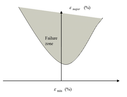
Figure 1. Generic Forming Limit Diagram (FLD)

Spalling with Johnson-Cook Failure Model

In this model, the Johnson-Cook failure model is combined to a Spalling model where we take into account the spall of the material when the pressure achieves a minimum value Pmin. The deviatoric stresses are set to zero for compressive pressure. If the hydrostatic tension is computed, then the pressure is set to zero. The failure equations are the same as in Johnson-Cook model.

Bao-Xue Wierzbicki Failure Model

Bao-Xue-Wierzbicki model 5 represents a 3D fracture criterion which can be expressed by:(6)
ε ¯ f n = ε ¯ max n [ ε ¯ max n ε ¯ min n ] ( 1 ξ ¯ m ) 1/m MathType@MTEF@5@5@+= feaagKart1ev2aqatCvAUfeBSjuyZL2yd9gzLbvyNv2CaerbuLwBLn hiov2DGi1BTfMBaeXatLxBI9gBaerbd9wDYLwzYbItLDharqqtubsr 4rNCHbGeaGqiVu0Je9sqqrpepC0xbbL8F4rqqrFfpeea0xe9Lq=Jc9 vqaqpepm0xbba9pwe9Q8fs0=yqaqpepae9pg0FirpepeKkFr0xfr=x fr=xb9adbaqaaeGaciGaaiaabeqaamaabaabaaGcbaGafqyTduMbae badaWgaaWcbaGaamOzaaqabaGcdaahaaWcbeqaaiaad6gaaaGccqGH 9aqpcuaH1oqzgaqeamaaBaaaleaaciGGTbGaaiyyaiaacIhaaeqaaO WaaWbaaSqabeaacaWGUbaaaOGaeyOeI0YaamWaaeaacuaH1oqzgaqe amaaBaaaleaaciGGTbGaaiyyaiaacIhaaeqaaOWaaWbaaSqabeaaca WGUbaaaOGaeyOeI0IafqyTduMbaebadaWgaaWcbaGaciyBaiaacMga caGGUbaabeaakmaaCaaaleqabaGaamOBaaaaaOGaay5waiaaw2faam aabmaabaGaaGymaiabgkHiTiqbe67a4zaaraWaaWbaaSqabeaacaWG TbaaaaGccaGLOaGaayzkaaWaaWbaaSqabeaacaaIXaGaai4laiaad2 gaaaaaaa@596C@
(7)
ε ¯ max = C 1 e C 2 η ¯ MathType@MTEF@5@5@+= feaagKart1ev2aqatCvAUfeBSjuyZL2yd9gzLbvyNv2CaerbuLwBLn hiov2DGi1BTfMBaeXatLxBI9gBaerbd9wDYLwzYbItLDharqqtubsr 4rNCHbGeaGqiVu0Je9sqqrpepC0xbbL8F4rqqrFfpeea0xe9Lq=Jc9 vqaqpepm0xbba9pwe9Q8fs0=yqaqpepae9pg0FirpepeKkFr0xfr=x fr=xb9adbaqaaeGaciGaaiaabeqaamaabaabaaGcbaGafqyTduMbae badaWgaaWcbaGaciyBaiaacggacaGG4baabeaakiabg2da9iaadoea daWgaaWcbaGaaGymaaqabaGccaWGLbWaaWbaaSqabeaacqGHsislca WGdbWaaSbaaWqaaiaaikdaaeqaaSGafq4TdGMbaebaaaaaaa@4303@
(8)
ε ¯ min = C 3 e C 4 η ¯ MathType@MTEF@5@5@+= feaagKart1ev2aqatCvAUfeBSjuyZL2yd9gzLbvyNv2CaerbuLwBLn hiov2DGi1BTfMBaeXatLxBI9gBaerbd9wDYLwzYbItLDharqqtubsr 4rNCHbGeaGqiVu0Je9sqqrpepC0xbbL8F4rqqrFfpeea0xe9Lq=Jc9 vqaqpepm0xbba9pwe9Q8fs0=yqaqpepae9pg0FirpepeKkFr0xfr=x fr=xb9adbaqaaeGaciGaaiaabeqaamaabaabaaGcbaGafqyTduMbae badaWgaaWcbaGaciyBaiaacMgacaGGUbaabeaakiabg2da9iaadoea daWgaaWcbaGaaG4maaqabaGccaWGLbWaaWbaaSqabeaacqGHsislca WGdbWaaSbaaWqaaiaaisdaaeqaaSGafq4TdGMbaebaaaaaaa@4305@
Where, C 1 , C 2 , C 3 , C 4 , γ and m MathType@MTEF@5@5@+= feaagKart1ev2aqatCvAUfeBSjuyZL2yd9gzLbvyNv2CaerbuLwBLn hiov2DGi1BTfMBaeXatLxBI9gBaerbd9wDYLwzYbItLDharqqtubsr 4rNCHbGeaGqiVu0Je9sqqrpepC0xbbL8F4rqqrFfpeea0xe9Lq=Jc9 vqaqpepm0xbba9pwe9Q8fs0=yqaqpepae9pg0FirpepeKkFr0xfr=x fr=xb9adbaqaaeGaciGaaiaabeqaamaabaabaaWcbaGaamyBaaaa@36EA@ are the material constants, n is the hardening parameter and η ¯ and ξ ¯ are defined as:
  • for solids:

    If Imoy=0:

    η ¯ = σ m σ V M ; ξ ¯ = 27 2 J 3 σ V M 3

    If Imoy=1:

    η ¯ = 0 ε p σ m σ V M d ε p ε p ξ ¯ = 0 ε p 27 J 3 2 σ V M 3 d ε p ε p
  • for shells:

    η ¯ = σ m σ V M ; ξ ¯ = 27 2 η ¯ ( η ¯ 2 1 3 )

Where,
σ m
Hydrostatic stress
σ V M
The von Mises stress
J 3 = s 1 s 2 s 3
Third invariant of principal deviatoric stresses


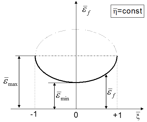
Figure 2. Graphical Representation of Bao-Xue-Wierzbicki Failure Criteria

Strain Failure Model

This failure model can be compared to the damage model in LAW27. When the principal tension strain ε 1 reaches ε t 1 , a damage factor D MathType@MTEF@5@5@+= feaagKart1ev2aqatCvAUfeBSjuyZL2yd9gzLbvyNv2CaerbuLwBLn hiov2DGi1BTfMBaeXatLxBI9gBaerbd9wDYLwzYbItLDharqqtubsr 4rNCHbGeaGqiVu0Je9sqqrpepC0xbbL8F4rqqrFfpeea0xe9Lq=Jc9 vqaqpepm0xbba9pwe9Q8fs0=yqaqpepae9pg0FirpepeKkFr0xfr=x fr=xb9adbaqaaeGaciGaaiaabeqaamaabaabaaGcbaGaamiraaaa@36C0@ is applied to reduce the stress, as shown in Figure 3. The element is ruptured when D MathType@MTEF@5@5@+= feaagKart1ev2aqatCvAUfeBSjuyZL2yd9gzLbvyNv2CaerbuLwBLn hiov2DGi1BTfMBaeXatLxBI9gBaerbd9wDYLwzYbItLDharqqtubsr 4rNCHbGeaGqiVu0Je9sqqrpepC0xbbL8F4rqqrFfpeea0xe9Lq=Jc9 vqaqpepm0xbba9pwe9Q8fs0=yqaqpepae9pg0FirpepeKkFr0xfr=x fr=xb9adbaqaaeGaciGaaiaabeqaamaabaabaaGcbaGaamiraaaa@36C0@ =1. In addition, the maximum strains ε t 1 and ε t 2 may depend on the strain rate by defining a scale function.


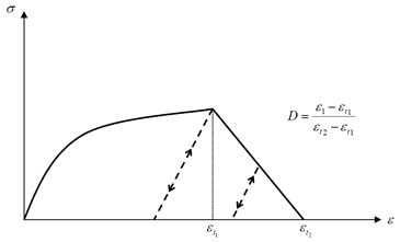
Figure 3. Strain Failure Model

Specific Energy Failure Model

When the energy per unit volume achieves the value E 1 , then the damage factor D MathType@MTEF@5@5@+= feaagKart1ev2aqatCvAUfeBSjuyZL2yd9gzLbvyNv2CaerbuLwBLn hiov2DGi1BTfMBaeXatLxBI9gBaerbd9wDYLwzYbItLDharqqtubsr 4rNCHbGeaGqiVu0Je9sqqrpepC0xbbL8F4rqqrFfpeea0xe9Lq=Jc9 vqaqpepm0xbba9pwe9Q8fs0=yqaqpepae9pg0FirpepeKkFr0xfr=x fr=xb9adbaqaaeGaciGaaiaabeqaamaabaabaaGcbaGaamiraaaa@36C0@ is introduced to reduce the stress. For the limit value E 2 , the element is ruptured. In addition, the energy values E 1 and E 2 may depend on the strain rate by defining a scale function.


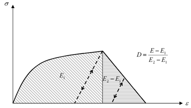
Figure 4. Strain Failure Model

XFEM Crack Initialization Failure Model

This failure model is available for Shell only.

In /FAIL/TBUTCHER, the failure mode criteria are written as:

For ductile materials, the cumulative damage parameter is:(9)
D = 0 t max ( 0 , ( σ σ r ) λ ) d t
Where,
σ r MathType@MTEF@5@5@+= feaagKart1ev2aqatCvAUfeBSjuyZL2yd9gzLbvyNv2CaerbuLwBLn hiov2DGi1BTfMBaeXatLxBI9gBaerbd9wDYLwzYbItLDharqqtubsr 4rNCHbGeaGqiVu0Je9sqqrpepC0xbbL8F4rqqrFfpeea0xe9Lq=Jc9 vqaqpepm0xbba9pwe9Q8fs0=yqaqpepae9pg0FirpepeKkFr0xfr=x fr=xb9adbaqaaeGaciGaaiaabeqaamaabaabaaGcbaGaeq4Wdm3aaS baaSqaaiaadkhaaeqaaaaa@38DD@
Fracture stress
σ
Maximum principal stress
λ
Material constant
t MathType@MTEF@5@5@+= feaagKart1ev2aaatCvAUfeBSjuyZL2yd9gzLbvyNv2CaerbuLwBLn hiov2DGi1BTfMBaeXatLxBI9gBaerbd9wDYLwzYbItLDharqqtubsr 4rNCHbGeaGqiVu0Je9sqqrpepC0xbbL8F4rqqrFfpeea0xe9Lq=Jc9 vqaqpepm0xbba9pwe9Q8fs0=yqaqpepae9pg0FirpepeKkFr0xfr=x fr=xb9adbaqaaeGaciGaaiaabeqaamaabaabaaGcbaGaamiDaaaa@36EF@
Time when shell cracks for initiation of a new crack within the structure
D MathType@MTEF@5@5@+= feaagKart1ev2aqatCvAUfeBSjuyZL2yd9gzLbvyNv2CaerbuLwBLn hiov2DGi1BTfMBaeXatLxBI9gBaerbd9wDYLwzYbItLDharqqtubsr 4rNCHbGeaGqiVu0Je9sqqrpepC0xbbL8F4rqqrFfpeea0xe9Lq=Jc9 vqaqpepm0xbba9pwe9Q8fs0=yqaqpepae9pg0FirpepeKkFr0xfr=x fr=xb9adbaqaaeGaciGaaiaabeqaamaabaabaaGcbaGaamiraaaa@36C0@
Another material constant called damage integral
For brittle materials, the damage parameter is:(10)
D ˙ = 1 K ( σ σ r ) a
(11)
σ r = σ 0 ( 1 D ) b
(12)
D = D + D ˙ Δ t
1 Argon A.S., J. Im, and Safoglu R., “Cavity formation from inclusions in ductile fracture”, Metallurgical Transactions, Vol. 6A, pp. 825-837, 1975.
2 Tuler F.R. and Butcher B.M., “A criteria for time dependence of dynamic fracture”, International Journal of Fracture Mechanics, Vol. 4, N°4, 1968.
3 Hashin, Z. and Rotem, A., “A Fatigue Criterion for Fiber Reinforced Materials”, Journal of Composite Materials, Vol. 7, 1973, pp. 448-464. 9.
4 Hashin, Z., “Failure Criteria for Unidirectional Fiber Composites”, Journal of Applied Mechanics, Vol. 47, 1980, pp. 329-334.
5 Wierzbicki T., “From crash worthiness to fracture; Ten years of research at MIT”, International Radioss User's Conference, Nice, June 2006.