Auto Contacts
The physics of contacts is involved in various phenomena, such as the impact of two billiard balls, the contact between two gears, the impact of a missile, the crash of a car, etc. While the physics of the contact itself is the same in all these cases, the main resulting phenomena are not.
In the case of billiard balls, it is the shock itself that is important and it will then be necessary to simulate perfectly the wave propagation. In the case of gears, it is the contact pressure that has to be evaluated precisely.
The quality of these simulations depends mainly on the quality of the models (spatial and temporal discretization) and on the choice of the integration scheme. In structural crash or vehicle crash simulations, the majority of the contacts result from the buckling of tubular structures and metal sheets. Modeling the structure using shell and plate finite elements, the physics of the contact cannot be described in a precise way. The reflection of the waves in the thickness is not captured and the distribution of contact pressures in the thickness is not taken into account. The peculiarity of the contacts occurring during the crash of a structure lies more in the complexity of the structural folding and the important number of contact zones than in the description of the impact or the contact itself.
During a contact between two solid bodies, the surface in contact is usually continuous and only slightly curved. On the other hand, during the buckling of a structure, the contacts, resulting from sheet folding, are many and complex. Globally, the contact is no longer between two identified surfaces, but in a surface impacting on itself. The algorithms able to describe this type of contact are “auto-impacting” algorithms. Especially adapted to shell structures, they still can be used to simulate the impact of the external surface of a solid (3D element) on itself.
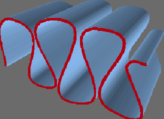
Figure 1.
- Capacity to make each point of the surface impact on itself
- Capacity to impact on both sides of a segment (internal and external)
- Possibility for a point of the surface to be wedged between an upper and a lower part
- Processing of very strong concavities (will complete folding)
- Reversibility of the contact, thereby authorizing unfolding after folding or the simulation of airbag deployment.
Contacts Modeling
- Contact nodes to nodes
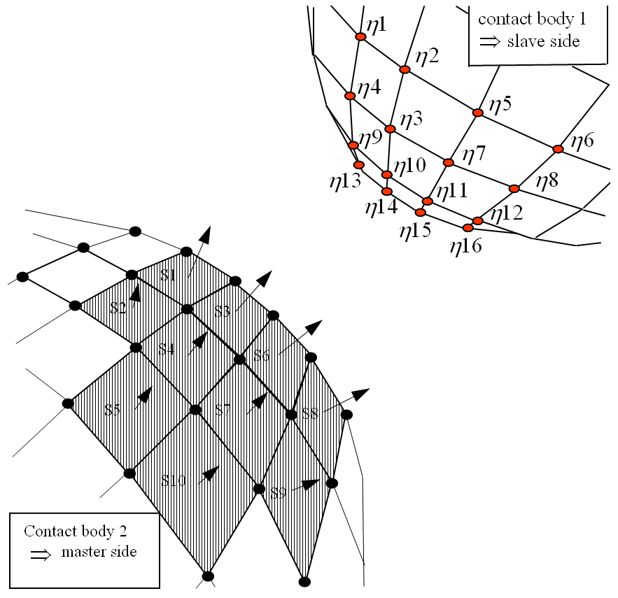
Figure 2. Contact Nodes to Surface
- Symmetrized contact nodes to surface
- The symmetrization of the previous formulation makes it possible to model a contact between two surfaces, as the group of nodes of the first surface can impact the second group and vice-versa.
-
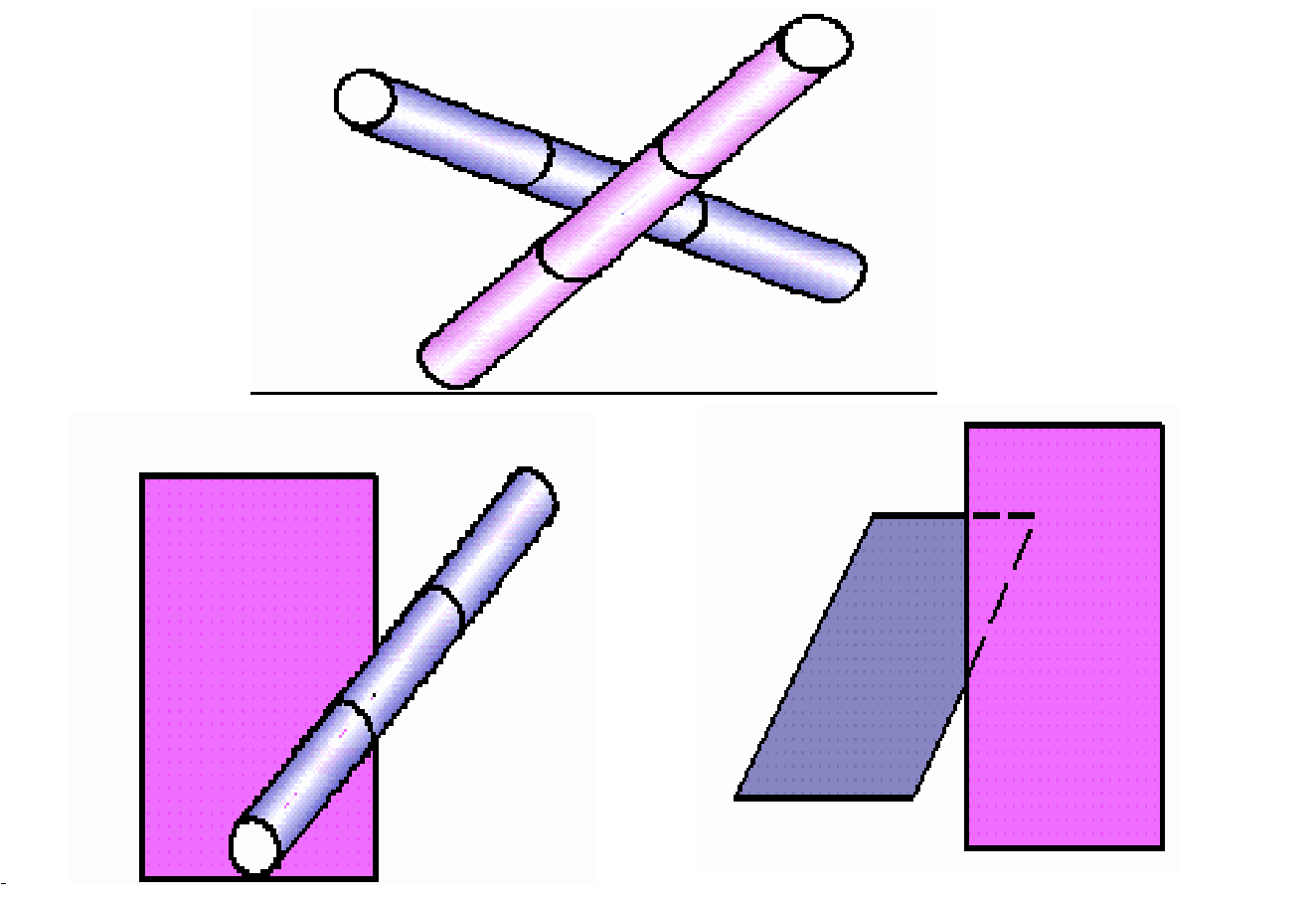
Figure 3. Contact Edges to Edges - Surface to surface contact
- Several approaches can be used to detect the contact between two surfaces. If the two surfaces are quadrangular, the exact calculation of the contact can be complex and quite expensive. An approximate solution may be made by combining the two previous formulations. By evaluating all the contacts of nodes to surface, as well as the edge to edge contacts, the only approximation is the partial consideration of the segment curvature.
Choice of a Formulation for Auto Impact
In the case of a surface impacting on itself, it is possible to use one of the previous formulations if considering certain specificities of the auto-contact. The choice of a formulation will depend on two essential criteria: the quality of the description of the contact and the robustness of the formulation. The selected formulation has to provide results that are as precise as possible in a normal operational situation, while still working in a satisfying way in extreme situations. The node-to-node method provides the best robustness, but the quality of the description is not sufficient enough to simulate in a realistic way those contacts occurring during the buckling of a structure.
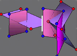
Figure 4.
Algorithms for Impact Candidates
During the impact of one part on another, it is possible to predict which node will impact on a certain segment. In the case of the buckling of a shell structure, such as a tube, it is impossible to predict where different contacts will occur. It is thus necessary to have a fairly general and powerful algorithm that is able to search for impact candidates.
The detail of the formulation of an algorithm, able to search for impact candidates, will depend on the choice of the contact formulation described in the previous chapter. In a node-to-node contact formulation, it is necessary to find for each node the closest node, whose distance is lower than a certain value. In the case of the edge-to-edge formulation, the search for neighboring entities concerns the edges and not the nodes. However, we should note that in some algorithms, the search for neighboring edges or segments is obtained by a node proximity calculation. Moreover, an algorithm designed to search for proximity of nodes can be adapted in order to transform it into a search for proximity of segments or even for a mixed proximity of nodes and segments.
- Direct search
- Topologically limited search
- Algorithms of sorting by boxes (bucket sort)
- Algorithms of fast sort (octree, quick sort)
When using direct search, at each cycle the distance is calculated from each entity (node, segment, edge) to all others. The quadratic cost (N*N) of this algorithm makes it unusable in case of auto-contact.
Topologically Limited Search
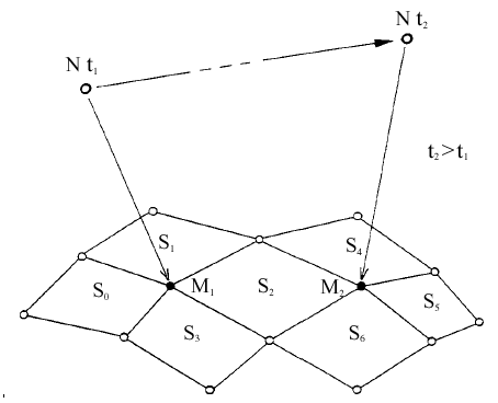
Figure 5.
It remains however necessary to do a complete search before the first cycle of calculation. We will also see that this algorithm presents significant restrictions that limit its use to sliding surfaces (it cannot be used for auto-impacting surfaces).
The cost of this algorithm is linear (N), except at the first cycle of computation, during which it is quadratic (N*N). The combination of this algorithm with one of the following two is also possible.
Bucket Sort
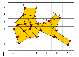
Figure 6.
In order to limit the memory space needed, we first count the number of nodes in each box, thereby making it possible to limit the filling of those boxes that are not empty. In the two-dimensional example shown above, nodes are arranged in the boxes as described in the following table. With this arrangement, the calculation of distances between nodes of the same box is not a problem. On the other hand, taking into account the nodes of neighboring boxes is not straightforward, especially in the horizontal direction (if the arrangement is first made vertically, as in this case). One solution is to consider three columns of boxes at a time. Another solution, more powerful but using more memory, would be for each box to contain the nodes already located there plus those belonging to neighboring boxes. This is shown in the third series of columns in the following table. Once this sorting has been performed, the last step is to calculate the distances between the different nodes of a box, followed by the distance between these nodes and those of the neighboring box. In box 0,3 for example, fifteen distances must be calculated.
11-14, 11-3, 11-8, 11-12, 11-15, 11-16, 11-17, 11-18, 14-3, 14-8,
14-12, 14-15, 14-16, 14-17, 14-18.
| Box | Nodes | Nodes of the Neighboring Box | ||||||||||||
|---|---|---|---|---|---|---|---|---|---|---|---|---|---|---|
| 0,0 | 26 | 21 | ||||||||||||
| 0,1 | 21 | 15 | 16 | 17 | 22 | 26 | ||||||||
| 0,2 | 16 | 8 | 11 | 12 | 14 | 15 | 17 | 21 | 22 | 26 | ||||
| 0,3 | 11 | 14 | 3 | 8 | 12 | 15 | 16 | 17 | 18 | |||||
| 1,1 | 22 | 15 | 16 | 17 | 19 | 21 | 23 | 26 | ||||||
| 1,2 | 15 | 17 | 8 | 11 | 12 | 13 | 14 | 18 | 16 | 19 | 21 | 22 | 23 | |
| 1,3 | 8 | 12 | 18 | 3 | 5 | 11 | 13 | 14 | 15 | 16 | 17 | 19 | ||
| 1,4 | 3 | 1 | 2 | 5 | 11 | 12 | 13 | 14 | 18 | |||||
| 1,5 | 1 | 2 | 3 | 5 | ||||||||||
| 2,1 | 23 | 15 | 17 | 19 | 22 | |||||||||
| 2,2 | 19 | 8 | 9 | 10 | 12 | 13 | 15 | 17 | 18 | 22 | 23 | |||
| 2,3 | 13 | 3 | 5 | 8 | 9 | 10 | 12 | 15 | 17 | 18 | 19 | |||
| 2,4 | 5 | 1 | 2 | 3 | 8 | 9 | 10 | 12 | 13 | 18 | ||||
| 2,5 | 2 | 1 | 3 | 5 | ||||||||||
| 3,3 | 9 | 10 | 4 | 5 | 6 | 13 | 19 | 20 | ||||||
| 4,1 | 24 | 20 | 25 | 27 | ||||||||||
| 4,2 | 20 | 9 | 10 | 24 | ||||||||||
| 4,4 | 4 | 6 | 9 | 10 | ||||||||||
| 5,0 | 25 | 27 | 24 | |||||||||||
In this example you have considered a search based on nodal proximity. It is possible to adapt this algorithm in order to arrange segments or even edges in the boxes. It will be necessary however to reserve more memory, for a segment can overlap several boxes.
Quick Sort
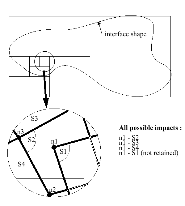
Figure 7. Possible Impact of Node n1
In order to illustrate the 3D quick sort, consider a search for node-segment proximity. At each step, space is successively divided into two equal parts, according to directions X, Y or Z. The group of nodes is thus separated into two subsets. We thereby obtain a tree organization with two branches per node. After each division, a check is made to determine whether the first of the two boxes must be divided. If so, it will be divided similar to the previous one. If not, the next branch is then checked. This recursive algorithm is identical to the regular fast sorting one.
The segments are also sorted using the spatial pivot. The result of the test can lead to three possibilities: the segment is on the left side of the pivot, on the right side of the pivot or astride the pivot. In the first two cases, the segments are treated similar to the nodes, but in the third situation, the segment is duplicated and placed on both sides.
- The box does not contain any nodes
- The box does not contain any segments
- The box contains sufficiently few elements that the calculation of distance of all the couples is more economical
- The dimension of the box is smaller than a threshold
Contact Processing
- Kinematic formulation of type main/secondary.
In a contact node to segment, the secondary node transmits its mass and force to the main segment and the segment transmits its speed to the node. This formulation is particularly adapted to an explicit integration scheme, provided that the nodes do not belong to a main segment. A node cannot be at the same time secondary and main. This approach then cannot be used in the case of auto-contact.
- The Lagrange multipliers ensure kinematic continuity at contact.
There is no restriction as in the previous formulation but the system of equations cannot be solved in an explicit way. The Lagrange multiplier matrix has to be reversed at each cycle of computation. In the case of auto-contact, the number of points in contact can become significant and this formulation then becomes quite expensive.
- Penalty methods do not ensure kinematic contact continuity, but they add springs at
the contact spots.
The first advantage to this formulation is its natural integration in an explicit code. Each contact is treated like an element and integrates itself perfectly into the code architecture, even if the programming is vectorial and parallel. Contrary to the kinematic formulations, the penalty method ensures the conservation of momentum and kinetic energy during impact.
The formulation used in Radioss is a penalty type formulation. The choice of the penalty factor is a major aspect of this method. In order to respect kinematic continuity, the penalty spring must be as rigid as possible. If the impedance of the interface becomes higher than those of the structures in contact, some numerical rebounds (high frequency) can occur. To ensure the stability of the integration diagram, without having additional constraints, this rigidity must be low. With a too low penalty, the penetration of the nodes becomes too strong and the geometrical continuity is no longer ensured.
The compromise selected consists in using a stiffness of the same order of magnitude than the stiffness of the elements in contact. This stiffness is nonlinear and increases with the penetration, so that a node is not allowed to cross the surface.
These choices provide a clear representation of physics, without numerical generation of noise, but require the contact stiffness in the calculation of the criteria of stability of the explicit scheme to be taken into account.
Contact Detection
After identifying the candidates for the impact, it is necessary to determine whether contact takes place and its precise localization. If for a formulation of node to node contact the detection of the contact is quite easy, it becomes more complex in the case of a node to segment or edge to edge contact. In the case of edge-to-edge contacts, a direct solution is possible if the segments are planar. If not, it is better to triangulate one of the segments, which would then turn it into a node-to-segment contact problem.
The search algorithm for candidates is uncoupled from the rest of the processing of the interfaces. This is not the case with regard to the detection, localization and processing of the contact. These last three tasks significantly overlap with each other so we will limit ourselves to the processing of the contact by penalty for simplicity.
In the case of contact between two solid bodies modeled with 3D finite elements, contact can only take place on the segments of the external surface. This external surface has a certain orientation and the impact of a node can come only from the outside. Most of the node-to-surface contact algorithms use this orientation to simplify detection of contact. In the case of impact of a two-dimensional structure modeled with shell or plate finite elements, contact is possible on both sides of the surface.
For an oriented surface, it is necessary to consider contacts of the positive dimension side of the surface on itself, contacts of the negative dimension side on itself, and the contact of the "positive" side on the "negative" one. This last situation, which is quite rare, can occur in the case of a surface rolled up into itself or during the impact of a twisted surface.
Node to Segment Contact
The use of a "gap" surrounding the segment is one way of providing physical thickness to the surface and makes it possible to distinguish the impacts on the top or on the lower part of the segment. The contact is activated if the node penetrates within the gap or if the distance from the node to the segment becomes smaller than the gap.
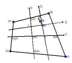
Figure 8.
The projected point is calculated using isoparametric coordinates for a quadrangular segment and barycentric coordinates for a triangular segment. In the case of any quadrangular segment, the exact calculation of these coordinates leads to a system of two quadratic equations that can be solved in an iterative way. The division of the quadrangular segment into four triangular segments makes it possible to work with a barycentric coordinate system and gives equations that can be solved in an analytical way.
From the isoparametric coordinates (, ) of the projected point (), we have all the necessary information for the detection and the processing of contact. The relations needed for the determination of and are: the vector is normal to the segment at the point ; and the normal to the segment is given by the vectorial product of the vectors and .
After bounding the isoparametric coordinates between +1 or -1, the distance from the node to the segment and the penetration are calculated:
A penalty force is deducted from this. It is applied to the node and distributed between the four nodes (, , , ) of the segment according to the following shape functions.
Edge to Edge Contact
The formulation of edge-to-edge contact is similar to that of node-to-segment contact. The gap surrounding each edge defines a cylindrical volume. The contact is detected if the distance between the two edges is smaller than the sum of the gaps of the two edges. The distance is then calculated as:
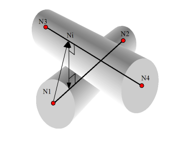
Figure 9.