Time Step Control Limitations
Many of the time step control options influence the solution results. The solution of the nonlinear dynamic response of a finite element system accurate is the numerical model correctly represents the physical model. The critical time step given for finite element system is determined by a theoretical approach in which the highest frequency of the discretized system controls this value. Therefore, the time step limitations are related to the model and cannot be changed without incidence on the quality of results.
Using the DEL option can significantly alter the model, since elements and nodes are removed without replacement. In fact, mass and/or volume is lost. Using either /DT/NODA/CST or /DT/INTER/CST will add mass to the model to allow mathematical solution. The added mass will increase the kinetic energy. This should be checked by the user to see if there is a significant effect. Switching to a small strain option using brick or shell elements also introduces errors as it was seen in Small Strain Formulation.
- Conservation of mass
- Conservation of energy
- Conservation of momentum dynamic equilibrium
The last one is generally respected as the equation of motion is resolved at each resolution cycle. However, in the case of adding masses especially when using /DT/NODA/CST option, it is useful to verify the momentum variation. The two other conservation laws are not explicitly satisfied. They should be checked a posteriori after computation to ensure the validity of the numerical model with respect to the physical problem.
Example: Time Step
Explicit Scheme Stability Condition
Where,
For non-divergence of Equation 7:
≥ : largest eigen value of is smaller than 1
≥
≥
≥ largest eigen value of
≥ < smallest eigen value of
Application
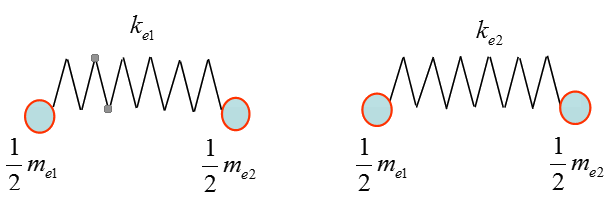
Figure 1.
Interface
Interfaces have stiffness but no mass:
- Impact speed