In direct integration method, at time the solutions for the prior steps are known and the solution
for the time is required next. The equations to relate displacements,
velocities and accelerations in a discrete time scale using the central difference time
integration algorithm are given in Central Difference Algorithm. They can be rewritten
as:(1)
For stability studies, aim to establish a recursive relationship to link the displacements
at three consecutive time steps:(2)
Where, is amplification matrix. A spectral analysis of this matrix
highlights the stability of the integration scheme.
The numerical algorithm is stable if and only if the radius spectral of is less than unity. In other words, when the module of all
eigen values of are smaller than unity, the numerical stability is
ensured.
The stability of a numerical scheme can be studied using the general form of the 2x2 matrix :(3)
Then, the equations are developed for the systems with or without damping. 1
The eigen values of are computed from the characteristic polynomial
equation:(4)
Where,
The eigen values are then obtained as:(5)
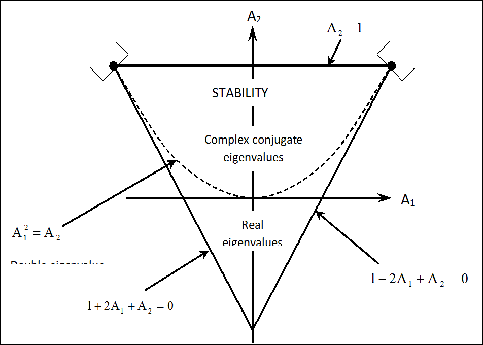
If , eigen values are complex conjugate; if , they are real and identical; if , they are real and distinct. You intend to define a stability
domain in the -space, where the spectral radius . The boundary of this domain is given by couples such as . Three cases are to be considered:
Roots are real and one of them is equal to 1:
You then have:(6)
This yields:(7)
The corresponding part of the boundary of the stability
domain is the segment analytically defined by and .
Roots are real and one of them is equal to -1:
You then have:(8)
This yields:(9)
In this case, the corresponding part of the boundary is the
segment given by and .
Roots are complex conjugate:
Their modulus is equal to 1. You then have, using :(10)
This yields:(11)
Since , you obtain:(12)
The corresponding part of the boundary is thus the segment
given by and .
The 3 segments introduced above define a closed
contour. Point is located inside this contour and in this case, . Since varies continuously with respect to and , you can conclude that the stability domain corresponds
to the interior of the contour. To precisely define the stability domain, you must
also have points leading to double eigen value of modulus 1, that is, the
intersections between the parabola and the boundary of the domain. This corresponds to
Points . Figure 1. Stability Domain
You can analytically summarize the description of the stability by means
of the following two sets of conditions:(13)
Numerical Stability of Undamped
Systems
The stability conditions developed in the previous section can be applied to a one
degree-of-freedom of a system without damping. The dynamic equilibrium equation at time is given by:(14)
Where, and are respectively the nodal mass and stiffness. is the external force at time . Rewriting the central difference time integration equations
from Equation 1, you
obtain:(15)
and:(16)
Substituting these equations into Equation 14, it
yields:(17)
This equation can be written as Equation 2. Then the
amplification matrix takes the expression:(18)
Where, is the angular frequency of the considered mode.
Comparing with Equation 3, you have and . Stability is then given by:(19)
The right inequality is always true if ≠ 0. For, the particular case of = 0, the scheme is unstable. However, the analytical solution for a
system with = 0 leads to an unbounded solution. The left inequality
implies:(20)
Numerical Stability with Viscous
Damping: Velocities at Time Steps
The dynamic equilibrium equation at time step is written as:(21)
Using the equations:(22)
Results in:(23)
For the velocity, write the equations:(24)
to obtain:(25)
Substituting these equations into Equation 21, the recurring
continuation equation on the displacement is written in the form:(26)
The equation can be rearranged to obtain the expression of the amplification
matrix:(27)
This yields and .
Stability is given by the set of conditions from Equation 13:(28)
The second expression is always verified for .
It is the same for the right inequality of the first expression. The left inequality of the
first expression leads to the condition on the time step:(29)
You find the same condition as in the undamped case, which echoes a conclusion given in
1. You may yet remark that damping has changed the strict
inequality into a large inequality, preventing from weak instability due to a double eigen
value of modulus unity.
It is important to note that the relation Equation 29 is obtained by using
the expression Equation 25 to compute nodal
velocities at time steps. However, in an explicit scheme generally the mid-step velocities and are used. This will be studied in the next section.
Numerical Stability with Viscous
Damping: Velocities at Mid Steps
Considering the case in which damping effects cannot be neglected, you still would like to
deal with decoupled equilibrium equations to be able to use essentially the same
computational procedure. Except for the case of full modal projection which is a very
expensive technique and practically unused, the damping matrix is not diagonal, contrary to . The computation of the viscous forces with the exact velocity
given by the integration algorithm requires the matrix to be inverted, which can harm the numerical performances. You
therefore often compute the viscous forces using the velocities at the preceding mid-step,
which are explicit. This leads to an equilibrium at step in the form:(30)
The integration algorithm immediately yields:(31)
The recurring continuation becomes:(32)
As above, you obtain the amplification matrix:(33)
You have in this case and .
Stability is again given by the set of conditions Equation 13:(34)
Right inequalities are always verified in both preceding expressions. Left inequalities now
lead to two conditions on the time step:(35)
Therefore, the critical time step depends not only to but also to the mass and the damping. However, the critical time step
depends only to when using the exact velocities to compute the viscous forces as
described in the previous section.
In the case of direct step-by-step time integration, it is necessary to evaluate the
damping matrix explicitly. The Rayleigh damping method assumes that the
matrix is computed by the following equation:(37)
Where,
Viscous damping matrix of the system
Mass matrix
Stiffness matrix
As described in the preceding sections, the computation of the viscous forces by using
velocities at time steps leads to obtain a non-diagonal matrix which should be inverted in the resolution procedure. To avoid
the high cost operations, generally the simplifications are made to obtain a diagonal
matrix. Substituting the Rayleigh equation into Equation 36 and using the mid-step
velocities for terms and at step nodal velocities for terms, the following expression is obtained:(38)
Studying the equilibrium of a node to obtain a one dimensional equation of motion,
write:(39)
Where,
Modal mass
Associated modal damping
Nodal stiffness
This leads to the following recurring continuation on the displacement:(40)
The amplification matrix is then:(41)
In this case, and .
Stability is obtained as before by means of the set of conditions from Equation 13:(42)
This again yields two conditions on the time step, coming from the left inequalities in
both expressions:(43)
It is equivalent to consider only the contribution in the damping for the computation of the time
step, which appears to be logical since the contribution is used with the exact velocity. It is
advantageous to separate the two contributions, restrictions of the time step then becoming
lighter. It can be shown that for the complete treatment of the Rayleigh damping using
mid-step velocities, the stability conditions can be given by:(44)
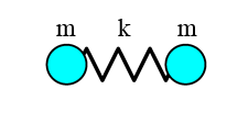
Example: Critical Time Step for a
Mass-Spring System
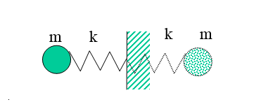
Figure 2.
Consider a free mass-spring system without damping. The governing differential equation can
be written as:
(a)
The element matrix expressions are given as:
;
The general solution is assumed in the form of:
(b)
Where, the angular frequency and the phase angle are common for all . and are the constants of integration to be determined from the
initial conditions of the motion and is a characteristic value (eigen value) of the system. Substituting (b)
into (a) yields:
(c)
The consistency of (c) for requires that:
=>
(d)
Assuming the following numerical values and , you have .
The critical time step of the system is given by Equation 20:
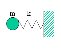
Example: Critical Time Step for
Dropping Body
A dropping body is studied in Body Drop Example with analytical and numerical approaches. As shown in Figure 5, the numerical results are closed to the analytical solution if you use a
step-by-step time discretization method with a constant time step . This value is less than the critical time step obtained
by:
Figure 3.
which may be computed as:
Therefore, the used time step in the Body Drop Example ensures the stability of the
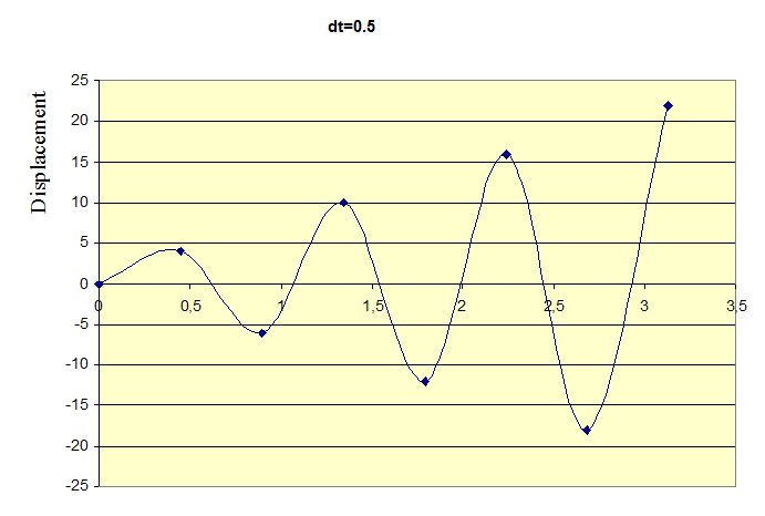
numerical scheme as it is less than the critical value. Now using the values higher than or
equal to the critical time step, the solution diverges towards the infinity as shown in
Figure 4. Figure 4. Numerical instability for Example Using Over Critical Time
Steps
It is worthwhile to comment that in a general explicit finite element program as Radioss, the critical time step is computed for an entire element (two
nodal masses and stiffness for spring element). In the case of dropping body example, the
mass-spring system can be compared by analogy to a two-node mass-spring system where the
global stiffness is twice softer. The critical time step is then computed using the nodal
time step of the entire element (refer to the following sections 1 for more details on the computation of nodal time step).
Figure 5.
1Hughes T.J.R., “Analysis of Transient Algorithms with Particular
Reference to Stability Behavior”, Computational Methods for Transient
Analysis, eds. T. Belytschko and T.J.R. Hugues, 67-155, North Holland,
1983.