Radioss uses elements with a lumped mass approach. This
reduces computational time considerably as no matrix inversion is necessary to compute
accelerations.
The integration scheme used by Radioss is based on the
central difference integration scheme which is conditionally stable, that is, the time step
must be small enough to assure that the solution does not grow boundlessly.
The
stability condition is given in the last sections. For a system without damping, it can be
written in a closed form:(1)
Where, is the highest angular frequency in the system:(2)
Where, and are respectively the stiffness and the mass matrices of the
system.
The time step restriction given by Equation 1 was derived
considering a linear system (Explicit Scheme Stability), but the result is also
applicable to nonlinear analysis since on a given step the resolution is linear. However, in
nonlinear analysis the stiffness properties change during the response calculation. These
changes in the material and the geometry influence the value of and in this way the critical value of the time step.
The above
point can be easily pointed out by using a nonlinear spring with increasing stiffness in
Body Drop Example. It can be shown that the
critical time step decreases when the spring becomes stiffer. Therefore, if a constant time
step close to the initial critical value is considered, a significant solution error is
accumulated over steps when the explicit central difference method is used.
Another
consideration in the time integration stability concerns the type of problem which is
analyzed. For example in the analysis of wave propagation, a large number of frequencies are
excited in the system. That is not always the case of structural dynamic problems. In a wave
shock propagation problem, the time step must be small enough in order to excite all
frequencies in the finite element mesh. This requires short time step so that the shock wave
does not miss any node when traveling through the mesh. It follows that the time step should
be limited by the following relation:(3)
Where,
Characteristic element length, representing the shortest road for a wave arriving on
a node to cross the element
Speed of sound in the material
Time step
The condition Equation 3 gives a severe time step
restriction with respect to stability time step, that is, . It can easily be shown that for a simple case of a bar
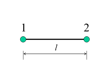
element, the two expressions Equation 3 and Equation 1 are equivalent. Figure 1. Bar Element
If a uniform linear-displacement bar element is considered, (Figure 2), and a lumped mass formulation at the nodes is used, the
highest frequency of this element can be obtained by a resolution of an eigen value
problem:(4)
(5)
For a lumped mass bar, you have:(6)
(7)
Where, and are respectively the nodal mass and stiffness of the
bar:(8)
which can be simplified with Equation 8 to
obtain:(11)
Where, is the speed of sound in the material and its expression is
given as:(12)
with the material density and the Young’s modulus. Combining Equation 11 and Equation 1, you
obtain:(13)
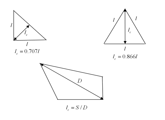
Figure 2. Element Characteristic Lengths
This relation is that of Equation 3 and shows that the
critical time step value in the explicit time integration of dynamic equation of motion can
be carried out by the interpretation of shock wave propagation in the material. This is
shown for the first time by Courant. 1 In spite of their works are limited to simple
cases, the same procedure can be used for different kinds of finite elements. The
characteristic lengths of the elements are found and Equation 3 is written for all
elements to find the most critical time step over a mesh. Regarding to the type (shape) of
element, the expression of characteristic length is different. Figure 2 shows some typical cases for elements with one integration
point.
1Courant R., Friedrichs K.O., and Levy H., “About the partial
Differenzensleichungen Bogdanova of Physics”, Math. A nn., Vol. 100, 32,
1928.