Body Drop Example

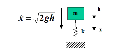
The question "how far can a body be dropped without incurring damage?" is frequently asked in the packaging manufacturing for transportation of particles. The problem is similar in landing of aircrafts. It can be studied by an analytical approach where the dropping body is modeled by a simple mass-spring system (Figure 1). If

h

is the dropping height,

m

and

k

the mass of the body and the stiffness representing the contact between the body and the ground, the equation of the motion can be represented by a simple one DOF differential equation as long as the spring remains in contact with floor:

(1)

m \ddot{x} + k x = m g

In this equation the damping effects are neglected to simplify the solution. The general solution of the differential equation is written as:(2)

x = A S i n ω t + B C o s ω t + C

Where, the constants A, B and C are determined by the initial conditions:(3)

At t=0 ≥ $x = 0$ , $\dot{x} = \sqrt{2 g h}$ , $\ddot{x} = g$

Where,

ω

is the natural frequency of the system: (4)

ω = \sqrt{\frac{k}{m}}

Introducing these initial solutions into Equation 3, the following result are obtained:(5)

x = \frac{\sqrt{2 g h}}{ω} S i n ω t + \frac{g}{ω^{2}} (1 - C o s ω t)

The same problem can be resolved by the numerical procedure explained in this section. Considering at first the following numerical values for the mass, the stiffness, the dropping height and the gravity:(6)

m = 1, k = 20, h = 1, g = 10

From Equation 1, the dynamic equilibrium equation or equation of motion is obtained as:(7)

\ddot{x} + 20 x = 10

Using a step-by-step time discretization method with a central difference algorithm, for a given known step

t_{n}

the unknown kinematic variables for the next step are given by Equation 7, Central Difference Algorithm, Equation 4 and Central Difference Algorithm, Equation 5:(8)

\begin{array}{l} {\ddot{x}}_{n} = 10 - 20 x_{n} \\ {\dot{x}}_{n + 1} = {\ddot{x}}_{n} Δ t + {\dot{x}}_{n} \\ x_{n + 1} = {\dot{x}}_{n} Δ t + x_{n} \end{array}

For the first time step the initial conditions are defined by Equation 3. Using a constant time step

Δ t = 0.1

the mass motion can be computed. It is compared to the analytical solution given by Equation 5 in Figure 2. The difference between the two results shows the time discretization error.