Methodology
The purpose of this section is to show the several steps for the generation of a proper Radioss ALE/CFD model.
CAD Cleaning
- Add surfaces to close volumes used by automatic tetrahedral mesh
- Add surface to control mesh progression
- Patch surfaces to prepare mesh zones
- Remove details whose size is smaller than what can be solved
- Remove line constraints on surfaces whenever possible
Mesh Generation
Figure 1. Tetrahedron Transformed to Hexahedron Mesh
- Outlet
- Inlet
- Non-reflective frontiers (NRF)
- Tubes
Of course, any other technique is suitable if generating hexahedron elements.
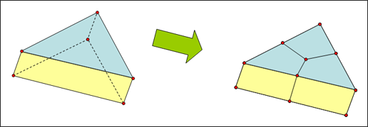
Figure 2. Split of a Pentahedron Element to Three Hexahedrons
Define Mesh Characteristics
- Velocity and pressure gradients: Near turbulent walls the mesh size is governed by the y+ value, which can range from 100 to 1000 or even higher (In pipes, y+ values as high as 8000 provide accurate results). From there, geometric progression is generally used toward coarser regions.
- Acoustic accuracy: A maximum size can be derived from the minimum wave length of interest. Generally use of 12 elements per wave length is acceptable.
Obviously the first condition will be governing region close to the obstacle or wall and the second will constrain the maximum size in the whole computational domain.
To build up a mesh, some trade-off is generally needed. The total time, , to be simulated can be evaluated as:
- Largest model size
- CPU = Ttot/dtc * Number of element * cpu/el/cycle
The generation of the mesh in order to perform the desired simulation has to be carefully defined according to two criteria and a trade-off between feasibility (CPU time available) and precision.
Criteria 1: Advection
- 10 elements minimum per vortex to be solved
- Local Strouhal number not exceeding 1/6 for the frequency range of "interest" in regions of
acoustic sources:
Str = f h/v < 1/6
For example: fmax =600 Hz, v=30m/s ≥ h ~ 8 mm
Criteria 2: Acoustic Propagation
- Critical in region away from acoustic sources
- Six elements per wave length along direction of propagation
For example: fmax = 600 Hz, c=300 m/s ≥ h ~ 8cm
Trade-off
- dt = Min (h) / c
- T = Ncycle * Nelem * Cost / cycle / elem
Practically, it is advised to perform a timing on a couple of cycles (do not forget to subtract the time of initialization) in order to know the cost per cycle of the simulation before launching a large simulation.
- Coarse mesh (all the computational domain except the immediate surroundings of the obstacle)
- Refined mesh (close to the obstacle)
- Inlet element (one row of elements)
- Outlet elements (one row of elements)
| Zone | Typical Size of Elements | Note |
|---|---|---|
| very fine | a | Chosen such as the obstacle is descretized with a minimum of 20 cells in each direction. |
| fine | 2a to 3a | |
| course | 4a to 6a | Make sure the course cells are appropriate for convection of the highest frequencies of interest. |
- Size of element < C / 10.f
- C
- Speed of sound in the fluid
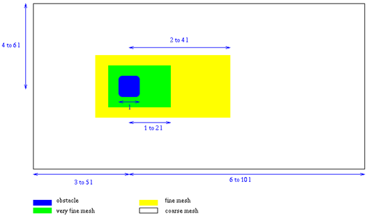
Figure 3. Number of Elements for Typical Mesh for CAA Problems (may vary for specific applications)
For problems with low Mach numbers (lower than 0.2), satisfactory results can be obtained under the quasi-compressibility assumption. This will save time on the computation. The compressibility implies that Navier-Stokes equations include wave equation. Then, acoustics and fluid flow can be treated at the same time, providing high numerical accuracy. Quasi-compressibility means, transport terms except in the momentum equation are neglected. Therefore, by reducing C1 in hydrodynamic material laws, the sound speed decreases and the time step increases (for example by dividing the C1 value by 10, the time step can be multiplied by 3).