Choice of Formulation
- Euler description
- Lagrangian description
The Arbitrary Lagrangian-Eulerian description was developed later to combine the advantages of the above classical kinematical descriptions, while minimizing their respective drawbacks as much as possible.
Euler Formulation
The Eulerian formulation is classical in fluid mechanics. The mesh is fixed and the material flows through the mesh. Equations are modified with respect to Lagrangian formulation in order to take into account the convective terms.
It can be activated for a specific part by a flag in material data:
/EULER/MAT/mat_ID
- mat_ID
- Identification number of the material to be set Eulerian
The treatment of moving boundaries and interfaces is difficult with Eulerian elements. The Eulerian formulation cannot be used in many cases where the boundaries of the domain move.
Lagrangian Formulation
The Lagrangian formulation is classical in structural analysis. The mesh is tied to the material points and follows the material deformation. No sliding between material (structure) and mesh is allowed. Loads and boundary conditions can easily be applied to the material points (nodes).
The Lagrangian description allows easy tracking of free surfaces and interfaces between different materials. However, when the structure is severely deformed, Lagrangian elements become similarly distorted since they follow the material deformation. Therefore, in those cases the accuracy and robustness of the Lagrangian simulations deteriorates severely.
This is the default formulation in Radioss, that is if a material is not defined as Eulerian (/EULER/MAT/mat_ID option), nor as ALE (/ALE/mat_ID option), this material is Lagrangian.
ALE Formulation
ALE stands for Arbitrary Lagrangian-Eulerian formulation. Material flows through an arbitrary moving mesh. Both the material and the mesh move with respect to the laboratory. It looks like a combination of Lagrangian and Eulerian formulations.
This formulation can be activated in Radioss for a specific part by a flag in the material data:
/ALE/MAT/mat_ID
- mat_ID
- Identification number of the material to be set in ALE
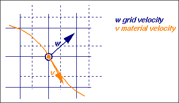
Figure 1. Arbitrary Grid Velocities and Displacements
In practice, built-in algorithms determine smooth grid deformation according to displacements of the ALE domain boundaries. Several algorithms are available (DONEA, SPRINGS, DISP, and ZERO).
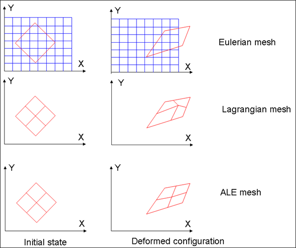
Figure 2. Eulerian, Lagrangian and ALE Meshes
Boundary nodes between ALE and Lagrangian materials must be set to Lagrangian: grid and material velocities are equal. Boundary nodes between ALE and Eulerian materials must have their grid velocity set to zero.