Force: FlexModal
Model ElementForce_FlexModal defines a distributed force on a flexible body.
Description
- A rigid body component that has a tendency to accelerate the flexible body that it is acting on, and,
- A modal component that has a tendency to deform the flexible body that it is acting on.
Format
<Force_FlexModal
       Id                                   = "integer"
       flex_body_id                         = "integer"
       {
               case_idx | case_id           = "integer"
               scale_expr                   = "string"
               [
                       usrsub_dll_name      = "string"
                       usrsub_fnc_name      = "string”
                       usrsub_param_string  = "User(par_1, ... par_N)"
                       |
                       Interpreter          = { "PYTHON" | "MATLAB" }
                       script_name          = "string"
                       usrsub_fnc_name      = "string"
                       usrsub_param_string  = "User(par_1, ... par_N)"
               ]
               [
                       force_sub            = "TRUE" | "FALSE"
               ]
       }
/>
Attributes
- id
- Specifies the element identification number of the Force_FlexModal element. This number should be unique among all Force_FlexModal elements. This parameter is mandatory.
- flex_body_id
- Specifies the ID of the flexible body on which this force acts. This parameter is mandatory.
- case_idx
- Specifies the modal load case number that is used to define the shape of the distributed load. Load cases are stored in the XML input deck in a Reference_FlexData modeling element. A separate ModeLoad block within the Reference_FlexData contains all the load cases.
- case_id
- Specifies the modal load case ID that is used to define the shape of the distributed load. Load cases are stored in the XML input deck in a Reference_FlexData modeling element. A separate ModeLoad block within the Reference_FlexData contains all the load cases. The difference between an ID and an Index is that indices are required to be contiguous whereas IDs are not.
- scale_expr
- Specifies an expression evaluated to a scalar quantity. The load case is multiplied by the run-time value of the expression to generate the distributed load acting on the flexible body. scale_expr can be a constant, a function of time or a function of state. It is required to be continuous.
- usrsub_param_string
- This keyword defines a list of parameters that are passed from the data file to the user-written subroutine. Use this keyword only when a user-written subroutine is to be defined.
- usrsub_fnc_name
- This keyword specifies name of the function that contains the definition of the distributed force. This function may be written in Fortran, C, C++ or Python.
- usrsub_dll_name
- Specifies the path and name of the DLL or shared library containing the user subroutine. MotionSolve uses this information to load the user subroutine in the DLL at run time.
- force_sub
- A Boolean that specifies whether the user subroutine should return the actual force (TRUE) or a shape that is to be scaled (FALSE).
- interpreter
- Specifies the interpreted language that the user script is written in.
- script_name
- Specifies the path and name of the user-written script that contains the routine specified by usrsub_fnc_name.
Example
A distributed load acting on a rectangular plate is used as an example to explain how the process illustrated in Figure 5 is implemented. Figure 1 below is the schematic of the system to be analyzed.
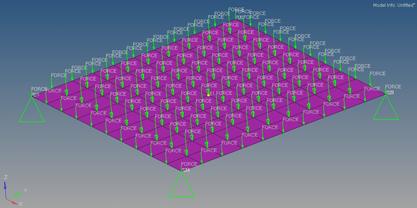
Figure 1. The Plate Model
The FE Input file corresponding to the plate and the distributed load is shown in Figure 2.
- Five interface nodes, four corner nodes (1, 11, 111, 121) and one center
node (61) were defined
ASET1 123 111 121 1 11 ASET1 123456 61 - Point load is applied on all nodes as follows
- Force of 253.36 N is applied along the negative Z-axis on the corner nodes
- Force of 506.72 N is applied along the negative Z-axis along the nodes on the edge of the plate
- Force of 1013.4 N is applied on all the internal nodes
FORCE          7      56       01.0     0.0     0.0     -506.72
FORCE          7      67       01.0     0.0     0.0     -506.72
FORCE          7      78       01.0     0.0     0.0     -506.72
FORCE          7      89       01.0     0.0     0.0     -506.72
FORCE          7     100       01.0     0.0     0.0     -506.72
FORCE          7      11       01.0     0.0     0.0     -253.36
FORCE          7       1       01.0     0.0     0.0     -253.36
FORCE          7     121       01.0     0.0     0.0     -253.36
FORCE          7     111       01.0     0.0     0.0     -253.36
- Craig-Bampton CMS option is selected with Force applied as LOADSET in
CMSMETH card
CMSMETH 8       CB              29
LOADSET BOTH    7
The total number of modes calculated for this case will be 48. There will be 4*3 + 1*6 static modes corresponding to the two sets of the ASET1 card defined. One additional static mode corresponding to the LOADSET and 29 dynamic modes as requested in the CMSMETH card.
Number of Modes = 4*3 + 1*6 + 1 + 29 = 48
- The load defined in the LOADSET portion of the CMSMETH card will be projected to the modal space and the modal load information will be written to the Flex H3D file for MBD solvers to use.
OptiStruct performs its analysis and generates a Flex H3D file that defines the modal flex body. In addition to the standard CMS data, the Flex H3D file also contains the distributed load - now defined in the modal domain. MotionSolve reads the Flex H3D file and places the modal load definition in the ModeLoad section of the Reference_FlexData block. This is shown in Figure 2.
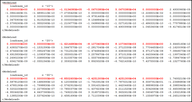
The ModeLoad section in the Reference_FlexData block of the MotionSolve XML input file specifies the different load-cases that are available for use. The plate model has 3 load cases. Each load case has an ID or an index.
- When the ModeLoad data is obtained from an Adams MNF, the load case index is available.
- When the data is obtained from a Flex H3D file, the load case ID is available. In this example, the load-case was obtained from OptiStruct, so a load case ID is available for use.
The load case represents a load shape, it needs to be scaled by a scale factor to obtain the true load on the plate. Each load case consists of 6+N numbers.
- The first 6 numbers, highlighted in yellow-red, are the rigid body loads. For the plate model, FZ, TX and TY are non-zero.
- The next N numbers are the contribution to equations of motion for each mode. The plate was characterized by 42 modes, so N=42 for this example.
Figure 3 shows the z-displacement of Node 61, which is located at the center of the plate. Since a constant load is acting on the plate and damping is included, the expectation should be that the oscillations of any node should eventually be dissipated. This is exactly what is seen.

Figure 3. The Z Displacement And Velocity Of Node 61 Compared To A Reference Result
Figure 4 shows the deformation contour of the plate at T=0.45s.

Figure 4. The Z Deformation Contour of the Plate
Comments
- Force_FlexModal allows you to apply a distributed load on a flexible body. The distributed load may be an aerodynamic load, liquid pressure, a thermal load, an electromagnetic force or any force generating mechanism that is spread out over the flexible body, such as non-uniform damping or visco-elasticity. It may be even be used to model a contact force between two bodies. In the last scenario, Force_FlexModal represents the distributed force acting on one of the flexible bodies involved in the contact.
- The force is defined in the modal domain because it is an
efficient method for defining the force and calculating its effects. However,
this requires that the transformation of the distributed load from the physical
domain, where the force is initially defined, to the modal domain be performed
in a finite element package.
The finite element package responsible for creating the flexible body generates the mode shapes through a process known as component mode synthesis. Since it knows about the modes of the flexible body it is able to transform a NODAL load description to a MODAL load description.
The process for creating distributed forces in HyperWorks is illustrated in Figure 5.

Figure 5. The Process For Creating And Analyzing Distributed Loads in HyperWorks - If we define
 as the mode shapes of the
flexible body, and
as the mode shapes of the
flexible body, and  as the Nodal load acting on
the flexible body, the equivalent Modal load on the flexible body
as the Nodal load acting on
the flexible body, the equivalent Modal load on the flexible body
 is defined
as:
is defined
as: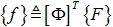
- Since
 contains only a subset of
the full set of modes describing the flexible body, the quantity
contains only a subset of
the full set of modes describing the flexible body, the quantity
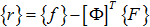 is lost in the Nodal to
Modal conversion. When the CMS method is used correctly, the residual,
is lost in the Nodal to
Modal conversion. When the CMS method is used correctly, the residual,  , is a small quantity.
 - The transformation from Nodal to Modal basis does not lose the resultant force that acts on the flexible body. The resultant force will tend to provide rigid body motion to the flexible body.
- The first six components of the load case or the load vector
returned by the user subroutine contain the resultant force. These are defined
as follows:
- 1 = Force acting along the X-axis of the LPRF Marker of the flexible body
- 2 = Force acting along the Y-axis of the LPRF Marker of the flexible body
- 3 = Force acting along the Z-axis of the LPRF Marker of the flexible body
- 4 = Torque acting about the X-axis of the LPRF Marker of the flexible body
- 5 = Torque acting about the Y-axis of the LPRF Marker of the flexible body
- 6 = Torque acting about the Z-axis of the LPRF Marker of the flexible body
- When the distributed force represents an internal load such as a thermal load or a modal damping force, the first six components (the rigid body components) of the load case are zero.
- Force_FlexModal is quite versatile. It
provides you with many options for defining the distributed load. These are
described below.
- Option-1: Scale factor defined in a time or state-dependent expression
This method can be used when the modal load shape has been parameterized in terms of quantities available in the multi-body model. In this scenario, you just need to specify the flexible body on which the modal force acts, the load case that you wish to use, and an expression defining the scale factor. The example below illustrates this option.
<Force_FlexModal id = "101" flex_body_id = "34" case_idx = "4" scale_expr = "Pi*Pitch(1015)*Vx(1015)*Vx(1015)" /> - Option-2: Scale factor defined in a user-subroutine
This method is used when the scale factor is not a simple expression as shown in option-1. In this case, the complex calculations for determining the scale factor may be embedded in a Python script or a compiled Fortran/C function. The example below illustrates how Force_FlexModal is specified in a Python script.
<Force_FlexModal
     id                    = "101"
     flex_body_id          = "34"
     usrsub_param_string   = "User(1015)"
     interpreter           = "Python"
     usrsub_fnc_name       = "Lift_and_Drag"
     script_name           = "/Users/MotionSolve/Example/lift.py"
     force_sub             = "FALSE"
/>
The user subroutine returns two quantities:- The load case index
- The scale factor
MotionSolve uses the above information to apply the distributed load to the flexible body. You are allowed to use SYSFNC and SYSARY to access the instantaneous state of the system and use it to define the scale factor.
- Option-3: Defining the distributed load shape and scale in a
user-subroutine This method is used when load shape is not available in the Flex-H3D file. This could be for a variety of reasons - one of these is that your finite element solver does not know how to generate a Flex-H3D file. The distributed load is calculated as:
 , where
q is the system
state, x the spatial
domain over which the distributed load acts and
t is the
independent variable, time.
, where
q is the system
state, x the spatial
domain over which the distributed load acts and
t is the
independent variable, time. The user subroutine returns two quantities:
- The scale factor, Scale(q,t). You are allowed to use SYSFNC and SYSARY to access the instantaneous state of the system and use it to define the scale factor.
- The load shape, Shape(x,t). The shape may
not be a function of the system states. It can only be
a function of the spatial domain and time.
MotionSolve uses the above information to apply the distributed load to the flexible body. The example below illustrates how Force_FlexModal is specified in the case when the user subroutine is written in a compiled language like Fortran, C or C++.
<Force_FlexModal
     id                    = "101"
     flex_body_id          = "34"
     usrsub_param_string   = "User(1015)"
     usrsub_fnc_name       = "Lift_and_Drag"
     usrsub_dll_name       = "/Users/MotionSolve/Example/lift.so"
     force_sub             = "FALSE"
/>
MotionSolve uses the above information to apply the distributed load to the flexible body. The example below illustrates how Force_FlexModal is specified in the case when the user subroutine is written in Python.
<Force_FlexModal
     id                    = "101"
     flex_body_id          = "34"
     usrsub_param_string   = "User(1015)"
     interpreter           = "Python"
     usrsub_fnc_name       = "Lift_and_Drag"
     script_name           = "/Users/MotionSolve/Example/lift.py"
     force_sub             = "FALSE"
/>
- The results are written to the H3D file and can be visualized using HyperView.
- Option-1: Scale factor defined in a time or state-dependent expression