Hill's Law for Orthotropic Plastic Shells

Hill's law models an anisotropic yield behavior. It can be considered as a generalization of von Mises yield criteria for anisotropic yield behavior.

The yield surface defined by Hill can be written in a general form:(1)

\begin{array}{l} F {(σ_{22} - σ_{33})}^{2} + G {(σ_{33} - σ_{11})}^{2} + H {(σ_{11} - σ_{22})}^{2} + 2 L σ_{23}^{2} + \\ 2 M σ_{31}^{2} + 2 N σ_{12}^{2} - 1 = 0 \end{array}

Where, the coefficients $F$ , $G$ , $H$ , $L$ , $M$ and $N$ are the constants obtained by the material tests in different orientations. The stress components $σ$ _1j are expressed in the Cartesian reference parallel to the three planes of anisotropy. Equation 1 is equivalent to von Mises yield criteria if the material is isotropic.

In a general case, the loading direction is not the orthotropic direction. In addition, we are concerned with the plane stress assumption for shell structures. In planar anisotropy, the anisotropy is characterized by different strengths in different directions in the plane of the sheet. The plane stress assumption will enable to simplify Equation 1, and write the expression of equivalent stress

σ_{e q}

as:(2)

σ_{e q} = \sqrt{A_{1} σ_{11}^{2} + A_{2} σ_{22}^{2} - A_{3} σ_{11} σ_{22} + A_{12} σ_{12}^{2}}

The coefficients

A_{1}

are determined using Lankford's anisotropy parameter

r_{α}

:(3)

\begin{array}{l} R = \frac{r_{00} + 2 r_{45} + r_{90}}{4}; H = \frac{R}{1 + R}; A_{1} = H (1 + \frac{1}{r_{00}}) \\ A_{2} = H (1 + \frac{1}{r_{90}}); A_{3} = 2 H; A_{12} = 2 H (r_{45} + 0.5) (\frac{1}{r_{00}} + \frac{1}{r_{90}}) \end{array}

Where, the Lankford's anisotropy parameters

r_{α}

are determined by performing a simple tension test at angle α to orthotropic direction 1:(4)

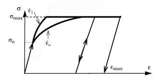
r_{α} = \frac{d ε_{α + \frac{π}{2}}}{d ε {}_{33}} = \frac{H + (2 N - F - G - 4 H) S i n^{2} α C o s^{2} α}{F S i n^{2} α + G C o s^{2} α}

The equivalent stress

σ_{e q}

is compared to the yield stress

σ_{y}

which varies in function of plastic strain

ε_{p}

and the strain rate

\dot{ε}

(LAW32):(5)

σ_{y} = a {(ε_{0} + ε_{p})}^{n} . \max {(\dot{ε}, {\dot{ε}}_{0})}^{m}

Therefore, the elastic limit is obtained by:(6)

σ_{0} = a {(ε_{0})}^{n} . {({\dot{ε}}_{0})}^{m}

The yield stress variation is shown in Figure 1.

The strain rates are defined at integration points. The maximum value is taken into account:(7)

\frac{d ε}{d t} = \max (\frac{d ε_{x}}{d t}, \frac{d ε_{y}}{d t}, 2 \frac{d}{d t} (ε_{x y}))

In Radioss, it is also possible to introduce the yield stress variation by a user-defined function (LAW43). Then, several curves are defined to take into account the strain rate effect.

It should be noted that as Hill's law is an orthotropic law, it must be used for elements with orthotropy properties as TYPE9 and TYPE10 in Radioss.

Anistropic Hill Material Law with MMC Fracture Model (LAW72)

This material law uses an anistropic Hill yield function along with an associated flow rule. A simple isotropic hardening model is used coupled with a modified Mohr fracture criteria. The yield condition is written as:

$φ (σ, σ_{y}) = σ_{H i l l} - σ_{y} = 0$

Where,

σ_{H i l l}

is the Equivalent Hill stress given as:

For 3D model (Solid)
$σ_{\begin{array}{l} H i l l \end{array}} = \sqrt{F {(σ_{y y} - σ_{z z})}^{2} + G {(σ_{z z} - σ_{x x})}^{2} + H {(σ_{x x} - σ_{y y})}^{2} + 2 L σ_{y z}^{2} + 2 M σ_{z x}^{2} + 2 N σ_{x y}^{2}}$
For Shell
$σ_{h i l l} = \sqrt{F σ_{y y}^{2} + G σ_{x x}^{2} + H {(σ_{x x} - σ_{y y})}^{2} + 2 N σ_{x y}^{2}}$

Where, $F$ , $G$ , $H$ , $N$ , $M$ , and $L$ are six Hill anisotropic parameters.

For the yield surface a modified swift law is employed to describe the isotropic hardening in the application of the plasticity models:

$σ_{y} = σ_{y}^{0} {(ε_{p}^{0} + ε_{p})}^{n}$

Where,

$σ_{y}^{0}$: Initial yield stress
$ε_{p}^{0}$: Initial equivalent plastic strain
$ε_{p}$: Equivalent plastic strain
$n$: Material constant

Modified Mohr fracture criteria

A damage accumulation is computed as:

$D = \int_{0}^{ε_{p}} \frac{d ε_{p}}{ε_{f} (θ, η)}$

Where,

ε_{f}

is a plastic strain fracture for the modified Mohr fracture criteria is given by:

Anisotropic 3D model
$ε_{f} = {\frac{σ_{y}^{0}}{C_{2}} [C_{3} + \frac{\sqrt{3}}{2 - \sqrt{3}} (1 - C_{3}) (\sec (\frac{θ π}{6}) - 1)] [\sqrt{\frac{1 + C_{1}^{2}}{3}} \cos (\frac{θ π}{6}) + C_{1} (η + \frac{1}{3} \sin (\frac{θ π}{6}))]}^{- \frac{1}{n}}$

with:

${\begin{matrix} θ = 1 - \frac{2}{π} \arccos ξ \\ ξ = \frac{27}{2} \frac{J_{3}}{σ_{V M}^{3}} \\ η = \frac{\frac{1}{3} (σ_{x x} + σ_{y y} + σ_{z z})}{σ_{V M}} \end{matrix}$

Where,

$J_{3}$

Third invariant of the deviatoric stress
2D Anisotropic Model
$ε_{f} = {\frac{σ_{y}^{0}}{C_{2}} f_{3} [(\sqrt{\frac{1 + C_{1}^{2}}{3}} f_{1}) + C_{1} (η + \frac{f_{2}}{3})]}^{- \frac{1}{n}}$

With:

${\begin{matrix} f_{1} = \cos {\frac{1}{3} \arcsin [- \frac{27}{2} η (η^{2} - \frac{1}{3})]} \\ f_{2} = \sin {\frac{1}{3} \arcsin [- \frac{27}{2} η (η^{2} - \frac{1}{3})]} \\ f_{3} = C_{3} + \frac{\sqrt{3}}{2 - \sqrt{3}} (1 - C_{3}) (\frac{1}{f_{1}} - 1) \end{matrix}$

Where,

$C_{1}$ , $C_{2}$ and $C_{3}$

Parameters for MMC fracture model

The fracture initiates when

D

= 1.

In order to represent realistic process of an element, a softening function

β

is introduced to reduce the deformation resistance. The yield surface is modified as:

$σ_{y} = β σ_{y}^{0} {(ε_{p}^{0} + ε_{p})}^{n}$

with $β = {(\frac{D_{c} - D}{D_{c} - 1})}^{m}$

Where,

$D_{c}$: Critical damage

We have crack propagation when $1 < D < D_{C}$ in this case $0 < β < 1$ is considered to reduce the yield surface otherwise the $β$ =1.

The element is deleted if $D \geq D_{c}$ .