Elastic-plastic Orthotropic Composite Shells

Two kinds of composite shells may be considered in the modeling:
  • Composite shells with isotropic layers
  • Composite shells with at least one orthotropic layer
The first case can be modeled by an isotropic material where the composite property is defined in element property definition as explained in Element Library. However, in the case of composite shell with orthotropic layers the definition of a convenient material law is needed. Two dedicated material laws for composite orthotropic shells exist in Radioss:
  • Material law COMPSH (25) with orthotropic elasticity, two plasticity models and brittle tensile failure,
  • Material law CHANG (15) with orthotropic elasticity, fully coupled plasticity and failure models.

These laws are described here. The description of elastic-plastic orthotropic composite laws for solids is presented in the next section.

Tensile Behavior

The tensile behavior is shown in Figure 2. The behavior starts with an elastic phase. Then, reached to the yield state, the material may undergo an elastic-plastic work hardening with anisotropic Tsai-Wu yield criteria. It is possible to take into account the material damage. The failure can occur in the elastic stage or after plastification. It is started by a damage phase then conducted by the formation of a crack. The maximum damage factor will allow these two phases to separate. The unloading can happen during the elastic, elastic-plastic or damage phase. The damage factor d MathType@MTEF@5@5@+= feaagKart1ev2aaatCvAUfeBSjuyZL2yd9gzLbvyNv2CaerbwvMCKf MBHbqefqvATv2CG4uz3bIuV1wyUbqedmvETj2BSbqefm0B1jxALjhi ov2DaebbnrfifHhDYfgasaacH8srps0lbbf9q8WrFfeuY=Hhbbf9v8 qqaqFr0xc9pk0xbba9q8WqFfea0=yr0RYxir=Jbba9q8aq0=yq=He9 q8qqQ8frFve9Fve9Ff0dmeaacaGacmGadaWaaiqacaabaiaafaaake aacaWGKbaaaa@39C0@ varies during deformation as in the case of isotropic material laws (LAW27). However, three damage factors are computed; two damage factors d 1 MathType@MTEF@5@5@+= feaagKart1ev2aaatCvAUfeBSjuyZL2yd9gzLbvyNv2CaerbuLwBLn hiov2DGi1BTfMBaeXatLxBI9gBaerbd9wDYLwzYbItLDharqqtubsr 4rNCHbGeaGqiVu0Je9sqqrpepC0xbbL8F4rqqrFfpeea0xe9Lq=Jc9 vqaqpepm0xbba9pwe9Q8fs0=yqaqpepae9pg0FirpepeKkFr0xfr=x fr=xb9adbaqaaeGaciGaaiaabeqaamaabaabaaGcbaGaamizamaaBa aaleaacaaIXaaabeaaaaa@37C6@ and d 2 MathType@MTEF@5@5@+= feaagKart1ev2aaatCvAUfeBSjuyZL2yd9gzLbvyNv2CaerbuLwBLn hiov2DGi1BTfMBaeXatLxBI9gBaerbd9wDYLwzYbItLDharqqtubsr 4rNCHbGeaGqiVu0Je9sqqrpepC0xbbL8F4rqqrFfpeea0xe9Lq=Jc9 vqaqpepm0xbba9pwe9Q8fs0=yqaqpepae9pg0FirpepeKkFr0xfr=x fr=xb9adbaqaaeGaciGaaiaabeqaamaabaabaaGcbaGaamizamaaBa aaleaacaaIXaaabeaaaaa@37C6@ for orthotropy directions and the other d 3 MathType@MTEF@5@5@+= feaagKart1ev2aaatCvAUfeBSjuyZL2yd9gzLbvyNv2CaerbuLwBLn hiov2DGi1BTfMBaeXatLxBI9gBaerbd9wDYLwzYbItLDharqqtubsr 4rNCHbGeaGqiVu0Je9sqqrpepC0xbbL8F4rqqrFfpeea0xe9Lq=Jc9 vqaqpepm0xbba9pwe9Q8fs0=yqaqpepae9pg0FirpepeKkFr0xfr=x fr=xb9adbaqaaeGaciGaaiaabeqaamaabaabaaGcbaGaamizamaaBa aaleaacaaIXaaabeaaaaa@37C6@ for delamination:(1) σ 11 = E 11 ( 1 d 1 ) ε 11 σ 22 = E 22 ( 1 d 2 ) ε 22 σ 12 = G 12 ( 1 d 1 ) ( 1 d 2 ) γ 12


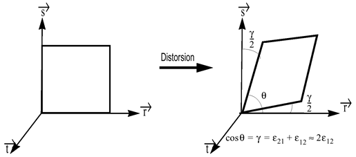
Figure 1. Shear Strain
Where, d 1 MathType@MTEF@5@5@+= feaagKart1ev2aaatCvAUfeBSjuyZL2yd9gzLbvyNv2CaerbuLwBLn hiov2DGi1BTfMBaeXatLxBI9gBaerbd9wDYLwzYbItLDharqqtubsr 4rNCHbGeaGqiVu0Je9sqqrpepC0xbbL8F4rqqrFfpeea0xe9Lq=Jc9 vqaqpepm0xbba9pwe9Q8fs0=yqaqpepae9pg0FirpepeKkFr0xfr=x fr=xb9adbaqaaeGaciGaaiaabeqaamaabaabaaGcbaGaamizamaaBa aaleaacaaIXaaabeaaaaa@37C6@ and d 2 MathType@MTEF@5@5@+= feaagKart1ev2aaatCvAUfeBSjuyZL2yd9gzLbvyNv2CaerbuLwBLn hiov2DGi1BTfMBaeXatLxBI9gBaerbd9wDYLwzYbItLDharqqtubsr 4rNCHbGeaGqiVu0Je9sqqrpepC0xbbL8F4rqqrFfpeea0xe9Lq=Jc9 vqaqpepm0xbba9pwe9Q8fs0=yqaqpepae9pg0FirpepeKkFr0xfr=x fr=xb9adbaqaaeGaciGaaiaabeqaamaabaabaaGcbaGaamizamaaBa aaleaacaaIXaaabeaaaaa@37C6@ are the tensile damages factors. The damage and failure behavior is defined by introduction of the following input parameters:
ε t 1
Tensile failure strain in direction 1
ε m 1
Maximum strain in direction 1
ε t 2
Tensile failure strain in direction 2
ε m 2
Maximum strain in direction 2
dmax
Maximum damage (residual stiffness after failure)


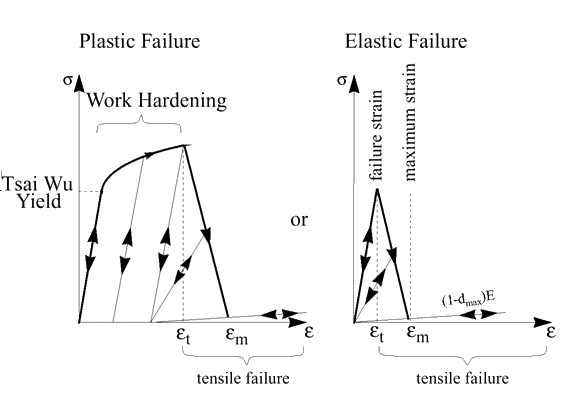
Figure 2. Tensile Behavior of Composite Shells

Delamination

The delamination equations are:(2) σ 31 = G 31 ( 1 d 3 ) γ 31 (3) σ 23 = G 23 ( 1 d 3 ) γ 23

Where, d 3 MathType@MTEF@5@5@+= feaagKart1ev2aaatCvAUfeBSjuyZL2yd9gzLbvyNv2CaerbuLwBLn hiov2DGi1BTfMBaeXatLxBI9gBaerbd9wDYLwzYbItLDharqqtubsr 4rNCHbGeaGqiVu0Je9sqqrpepC0xbbL8F4rqqrFfpeea0xe9Lq=Jc9 vqaqpepm0xbba9pwe9Q8fs0=yqaqpepae9pg0FirpepeKkFr0xfr=x fr=xb9adbaqaaeGaciGaaiaabeqaamaabaabaaGcbaGaamizamaaBa aaleaacaaIXaaabeaaaaa@37C6@ is the delamination damage factor. The damage evolution law is linear with respect to the shear strain.

Let γ= γ 31 2 + γ 23 2 then:(4)

for d 3 MathType@MTEF@5@5@+= feaagKart1ev2aaatCvAUfeBSjuyZL2yd9gzLbvyNv2CaerbuLwBLn hiov2DGi1BTfMBaeXatLxBI9gBaerbd9wDYLwzYbItLDharqqtubsr 4rNCHbGeaGqiVu0Je9sqqrpepC0xbbL8F4rqqrFfpeea0xe9Lq=Jc9 vqaqpepm0xbba9pwe9Q8fs0=yqaqpepae9pg0FirpepeKkFr0xfr=x fr=xb9adbaqaaeGaciGaaiaabeqaamaabaabaaGcbaGaamizamaaBa aaleaacaaIXaaabeaaaaa@37C6@ γ = γ i n i

for d 3 MathType@MTEF@5@5@+= feaagKart1ev2aaatCvAUfeBSjuyZL2yd9gzLbvyNv2CaerbuLwBLn hiov2DGi1BTfMBaeXatLxBI9gBaerbd9wDYLwzYbItLDharqqtubsr 4rNCHbGeaGqiVu0Je9sqqrpepC0xbbL8F4rqqrFfpeea0xe9Lq=Jc9 vqaqpepm0xbba9pwe9Q8fs0=yqaqpepae9pg0FirpepeKkFr0xfr=x fr=xb9adbaqaaeGaciGaaiaabeqaamaabaabaaGcbaGaamizamaaBa aaleaacaaIXaaabeaaaaa@37C6@ =1 ⇒ γ = γ max

Plastic Behavior

The plasticity model is based on the Tsai-Wu criterion 1 which enable to model the yield and failure phases. (5) F ( σ ) = F 1 σ 1 + F 2 σ 2 + F 11 σ 1 2 + F 22 σ 2 2 + F 44 σ 12 2 + 2 F 12 σ 1 σ 2
Where,(6) F 1 = 1 σ 1 y c + 1 σ 1 y t (7) F 22 = 1 σ 2 y c σ 2 y t (8) F 2 = 1 σ 2 y c + 1 σ 2 y t (9) F 44 = 1 σ 12 y c σ 12 y t (10) F 11 = 1 σ 1 y c σ 1 y t (11) F 12 = α 2 F 11 F 22
Where, α is the reduction factor. The six other parameters are the yield stresses in tension and compression for the orthotropy directions which can be obtained uniaxial loading tests:
σ 1 y t
Tension in direction 1 of orthotropy
σ 2 y t
Tension in direction 2 of orthotropy
σ 1 y c
Compression in direction 1 of orthotropy
σ 2 y c
Compression in direction 2 of orthotropy
σ 12 y c
Compression in direction 12 of orthotropy
σ 12 y t
Tension in direction 12 of orthotropy
The Tsai-Wu criteria are used to determine the material behavior: (12)
  • F ( σ ) < 1 : elastic state
  • F ( σ ) = 1 : plastic admissible state
  • F ( σ ) > 1 : plastically inadmissible stresses
For F ( σ ) = 1 the cross-sections of Tsai-Wu function with the planes of stresses in orthotropic directions is shown in Figure 3.


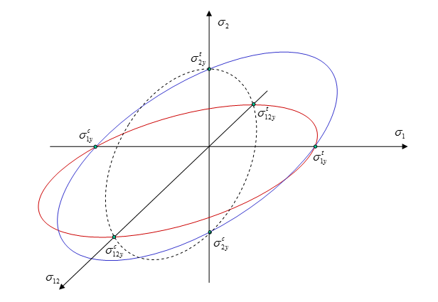
Figure 3. Cross-sections of Tsai-Wu Yield Surface For F ( σ ) = 1
If F ( σ ) > 1 , the stresses must be projected on the yield surface to satisfy the flow rule. F ( σ ) is compared to a maximum value F ( W p ) MathType@MTEF@5@5@+= feaagKart1ev2aaatCvAUfeBSjuyZL2yd9gzLbvyNv2CaerbuLwBLn hiov2DGi1BTfMBaeXatLxBI9gBaerbd9wDYLwzYbItLDharqqtubsr 4rNCHbGeaGqiVu0Je9sqqrpepC0xbbL8F4rqqrFfpeea0xe9Lq=Jc9 vqaqpepm0xbba9pwe9Q8fs0=yqaqpepae9pg0FirpepeKkFr0xfr=x fr=xb9adbaqaaeGaciGaaiaabeqaamaabaabaaGcbaGaamOramaabm aabaGaam4vamaaBaaaleaacaWGWbaabeaaaOGaayjkaiaawMcaaaaa @3A51@ varying in function of the plastic work W p MathType@MTEF@5@5@+= feaagKart1ev2aaatCvAUfeBSjuyZL2yd9gzLbvyNv2CaerbuLwBLn hiov2DGi1BTfMBaeXatLxBI9gBaerbd9wDYLwzYbItLDharqqtubsr 4rNCHbGeaGqiVu0Je9sqqrpepC0xbbL8F4rqqrFfpeea0xe9Lq=Jc9 vqaqpepm0xbba9pwe9Q8fs0=yqaqpepae9pg0FirpepeKkFr0xfr=x fr=xb9adbaqaaeGaciGaaiaabeqaamaabaabaaGcbaGaam4vamaaBa aaleaacaWGWbaabeaaaaa@37F3@ during work hardening phase:(13) F ( σ ) = F ( W p ) = 1 + b W p n
Where,
b MathType@MTEF@5@5@+= feaagKart1ev2aaatCvAUfeBSjuyZL2yd9gzLbvyNv2CaerbuLwBLn hiov2DGi1BTfMBaeXatLxBI9gBaerbd9wDYLwzYbItLDharqqtubsr 4rNCHbGeaGqiVu0Je9sqqrpepC0xbbL8F4rqqrFfpeea0xe9Lq=Jc9 vqaqpepm0xbba9pwe9Q8fs0=yqaqpepae9pg0FirpepeKkFr0xfr=x fr=xb9adbaqaaeGaciGaaiaabeqaamaabaabaaGcbaGaamOyaaaa@36DD@
Hardening parameter
n MathType@MTEF@5@5@+= feaagKart1ev2aaatCvAUfeBSjuyZL2yd9gzLbvyNv2CaerbuLwBLn hiov2DGi1BTfMBaeXatLxBI9gBaerbd9wDYLwzYbItLDharqqtubsr 4rNCHbGeaGqiVu0Je9sqqrpepC0xbbL8F4rqqrFfpeea0xe9Lq=Jc9 vqaqpepm0xbba9pwe9Q8fs0=yqaqpepae9pg0FirpepeKkFr0xfr=x fr=xb9adbaqaaeGaciGaaiaabeqaamaabaabaaGcbaGaamOyaaaa@36DD@
Hardening exponent
Therefore, the plasticity hardening is isotropic as illustrated in Figure 4.


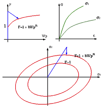
Figure 4. Isotropic Plasticity Hardening

Failure Behavior

The Tsai-Wu flow surface is also used to estimate the material rupture by means of two variables:
  • plastic work limit W p max ,
  • maximum value of yield function F max MathType@MTEF@5@5@+= feaagKart1ev2aaatCvAUfeBSjuyZL2yd9gzLbvyNv2CaerbwvMCKf MBHbqefqvATv2CG4uz3bIuV1wyUbqedmvETj2BSbqefm0B1jxALjhi ov2DaebbnrfifHhDYfgasaacH8srps0lbbf9q8WrFfeuY=Hhbbf9v8 qqaqFr0xc9pk0xbba9q8WqFfea0=yr0RYxir=Jbba9q8aq0=yq=He9 q8qqQ8frFve9Fve9Ff0dmeaacaGacmGadaWaaiqacaabaiaafaaake GabaaVqiaadAeadaWgaaWcbaGaciyBaiaacggacaGG4baabeaaaaa@3D71@
If one of the two conditions is satisfied, the material is ruptured. The evolution of yield surface during work hardening of the material is shown in Figure 5.


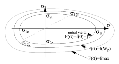
Figure 5. Evolution of Tsai-Wu Yield Surface
The model will allow the simulation of the brittle failure by formation of cracks. The cracks can either be oriented parallel or perpendicular to the orthotropic reference frame (or fiber direction), as shown in Figure 6. For plastic failure, if the plastic work W p MathType@MTEF@5@5@+= feaagKart1ev2aaatCvAUfeBSjuyZL2yd9gzLbvyNv2CaerbwvMCKf MBHbqefqvATv2CG4uz3bIuV1wyUbqedmvETj2BSbqefm0B1jxALjhi ov2DaebbnrfifHhDYfgasaacH8srps0lbbf9q8WrFfeuY=Hhbbf9v8 qqaqFr0xc9pk0xbba9q8WqFfea0=yr0RYxir=Jbba9q8aq0=yq=He9 q8qqQ8frFve9Fve9Ff0dmeaacaGacmGadaWaaiqacaabaiaafaaake aacaWGxbWaaSbaaSqaaiaadchaaeqaaaaa@3AD4@ is larger than the maximum value W p max for a given element, then the element is considered to be ruptured. However, for a multi-layer shell, several criteria may be considered to model a total failure. The failure may happen:
  • If W p > W p max for one layer,
  • If W p > W p max for all layers,
  • If W p > W p max or tensile failure in direction 1 for each layer,
  • If W p > W p max or tensile failure in direction 2 for each layer,
  • If W p > W p max or tensile failure in directions 1 and 2 for each layer,
  • If W p > W p max or tensile failure in direction 1 for all layers,
  • If W p > W p max or tensile failure in direction 2 for all layers,
  • If W p > W p max or tensile failure in directions 1 and 2 for each layer.
The last two cases are the most physical behaviors; but the use of failure criteria depends, at first, to the analyst’s choice. In Radioss the flag Ioff defines the used failure criteria in the computation.


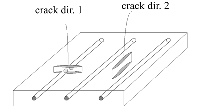
Figure 6. Crack Orientation

In practice, the use of brittle failure model allows to estimate correctly the physical behavior of a large rang of composites. But on the other hand, some numerical oscillations may be generated due to the high sensibility of the model. In this case, the introduction of an artificial material viscosity is recommended to stabilize results. In addition, in brittle failure model, only tension stresses are considered in cracking procedure.

The ductile failure model allows plasticity to absorb energy during a large deformation phase. Therefore, the model is numerically more stable. This is represented by CRASURV model in Radioss. The model makes also possible to take into account the failure in tension, compression and shear directions.

Strain Rate Effect

The strain rate is taken into account within the modification of Plastic Behavior, Equation 13 which acts through a scale factor:(14) F ( W p , ε ˙ ) = ( 1 + b ( W p W p r e f ) n ) ( 1 + c ln ( ε ˙ ε ˙ 0 ) )
Where,
W p MathType@MTEF@5@5@+= feaagKart1ev2aaatCvAUfeBSjuyZL2yd9gzLbvyNv2CaerbwvMCKf MBHbqefqvATv2CG4uz3bIuV1wyUbqedmvETj2BSbqefm0B1jxALjhi ov2DaebbnrfifHhDYfgasaacH8srps0lbbf9q8WrFfeuY=Hhbbf9v8 qqaqFr0xc9pk0xbba9q8WqFfea0=yr0RYxir=Jbba9q8aq0=yq=He9 q8qqQ8frFve9Fve9Ff0dmeaacaGacmGadaWaaiqacaabaiaafaaake aacaWGxbWaaSbaaSqaaiaadchaaeqaaaaa@3AD4@
Plastic work
W p r e f
Reference plastic work
b MathType@MTEF@5@5@+= feaagKart1ev2aaatCvAUfeBSjuyZL2yd9gzLbvyNv2CaerbuLwBLn hiov2DGi1BTfMBaeXatLxBI9gBaerbd9wDYLwzYbItLDharqqtubsr 4rNCHbGeaGqiVu0Je9sqqrpepC0xbbL8F4rqqrFfpeea0xe9Lq=Jc9 vqaqpepm0xbba9pwe9Q8fs0=yqaqpepae9pg0FirpepeKkFr0xfr=x fr=xb9adbaqaaeGaciGaaiaabeqaamaabaabaaGcbaGaamOyaaaa@36DD@
Plastic hardening parameter
n MathType@MTEF@5@5@+= feaagKart1ev2aaatCvAUfeBSjuyZL2yd9gzLbvyNv2CaerbuLwBLn hiov2DGi1BTfMBaeXatLxBI9gBaerbd9wDYLwzYbItLDharqqtubsr 4rNCHbGeaGqiVu0Je9sqqrpepC0xbbL8F4rqqrFfpeea0xe9Lq=Jc9 vqaqpepm0xbba9pwe9Q8fs0=yqaqpepae9pg0FirpepeKkFr0xfr=x fr=xb9adbaqaaeGaciGaaiaabeqaamaabaabaaGcbaGaamOyaaaa@36DD@
Plastic hardening exponent
c MathType@MTEF@5@5@+= feaagKart1ev2aaatCvAUfeBSjuyZL2yd9gzLbvyNv2CaerbuLwBLn hiov2DGi1BTfMBaeXatLxBI9gBaerbd9wDYLwzYbItLDharqqtubsr 4rNCHbGeaGqiVu0Je9sqqrpepC0xbbL8F4rqqrFfpeea0xe9Lq=Jc9 vqaqpepm0xbba9pwe9Q8fs0=yqaqpepae9pg0FirpepeKkFr0xfr=x fr=xb9adbaqaaeGaciGaaiaabeqaamaabaabaaGcbaGaamOyaaaa@36DD@
Strain rate coefficient (equal to zero for static loading)
The last equation implies the growing of the Tsai-Wu yield surface when the dynamic effects are increasing. The effects of strain rate are illustrated in Figure 7.


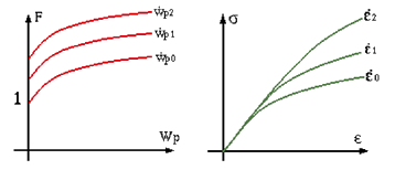
Figure 7. Strain Rate Effect in Work Hardening

CRASURV Model

The CRASURV model is an improved version of the former law based on the standard Tsai-Wu criteria. The main changes concern the expression of the yield surface before plastification and during work hardening. First, in CRASURV model the coefficient F 44 MathType@MTEF@5@5@+= feaagKart1ev2aaatCvAUfeBSjuyZL2yd9gzLbvyNv2CaerbuLwBLn hiov2DGi1BTfMBaeXatLxBI9gBaerbd9wDYLwzYbItLDharqqtubsr 4rNCHbGeaGqiVu0Je9sqqrpepC0xbbL8F4rqqrFfpeea0xe9Lq=Jc9 vqaqpepm0xbba9pwe9Q8fs0=yqaqpepae9pg0FirpepeKkFr0xfr=x fr=xb9adbaqaaeGaciGaaiaabeqaamaabaabaaGcbaGaamOramaaBa aaleaacaaI0aGaaGinaaqabaaaaa@3869@ in Plastic Behavior, Equation 5 depends only on one input parameter:(15) F 44 ( W p * , ε ˙ ) = 1 σ 12 ( W p * , ε ˙ ) σ 12 ( W p * , ε ˙ )

With σ 12 ( W p * , ε ˙ ) = σ 12 y ( 1 + b 12 ( W p * ) n 12 ) ( 1 + c 12 ln ( ε ˙ ε ˙ 0 ) )

Another modification concerns the parameters F ij MathType@MTEF@5@5@+= feaagKart1ev2aaatCvAUfeBSjuyZL2yd9gzLbvyNv2CaerbuLwBLn hiov2DGi1BTfMBaeXatLxBI9gBaerbd9wDYLwzYbItLDharqqtubsr 4rNCHbGeaGqiVu0Je9sqqrpepC0xbbL8F4rqqrFfpeea0xe9Lq=Jc9 vqaqpepm0xbba9pwe9Q8fs0=yqaqpepae9pg0FirpepeKkFr0xfr=x fr=xb9adbaqaaeGaciGaaiaabeqaamaabaabaaGcbaGaamOramaaBa aaleaacaWGPbGaamOAaaqabaaaaa@38CA@ in Plastic Behavior, Equation 5 which are expressed now in function of plastic work and plastic work rate as in Strain Rate Effect, Equation 14:(16) F ( W p * ) = F 1 ( W p * , ε ˙ ) σ 1 + F 2 ( W p * , ε ˙ ) σ 2 + F 11 ( W p * , ε ˙ ) σ 1 2 + F 22 ( W p * , ε ˙ ) σ 2 2 + 2 F 12 ( W p * , ε ˙ ) σ 1 σ 2 + F 44 ( W p * , ε ˙ ) σ 12 2

With

F i ( W p * , ε ˙ ) = 1 σ i c ( W p * , ε ˙ ) + 1 σ i t ( W p * , ε ˙ ) ( i MathType@MTEF@5@5@+= feaagKart1ev2aaatCvAUfeBSjuyZL2yd9gzLbvyNv2CaerbuLwBLn hiov2DGi1BTfMBaeXatLxBI9gBaerbd9wDYLwzYbItLDharqqtubsr 4rNCHbGeaGqiVu0Je9sqqrpepC0xbbL8F4rqqrFfpeea0xe9Lq=Jc9 vqaqpepm0xbba9pwe9Q8fs0=yqaqpepae9pg0FirpepeKkFr0xfr=x fr=xb9adbaqaaeGaciGaaiaabeqaamaabaabaaGcbaGaamyAaaaa@36E4@ =12)

F i i ( W p * , ε ˙ ) = 1 σ i c ( W p * , ε ˙ ) σ i t ( W p * , ε ˙ ) ( i MathType@MTEF@5@5@+= feaagKart1ev2aaatCvAUfeBSjuyZL2yd9gzLbvyNv2CaerbuLwBLn hiov2DGi1BTfMBaeXatLxBI9gBaerbd9wDYLwzYbItLDharqqtubsr 4rNCHbGeaGqiVu0Je9sqqrpepC0xbbL8F4rqqrFfpeea0xe9Lq=Jc9 vqaqpepm0xbba9pwe9Q8fs0=yqaqpepae9pg0FirpepeKkFr0xfr=x fr=xb9adbaqaaeGaciGaaiaabeqaamaabaabaaGcbaGaamyAaaaa@36E4@ =12)

F 12 ( W p * , ε ˙ ) = α 2 F 11 ( W p * , ε ˙ ) F 22 ( W p * , ε ˙ )

F 44 ( W p * , ε ˙ ) = 1 σ 12 ( W p * , ε ˙ ) σ 12 ( W p * , ε ˙ )

And(17) σ i t ( W p * , ε ˙ ) = σ i y t ( 1 + b i t ( W p * ) n i t ) ( 1 + c i t ln ( ε ˙ ε ˙ 0 ) ) MathType@MTEF@5@5@+= feaagKart1ev2aaatCvAUfeBSjuyZL2yd9gzLbvyNv2CaerbwvMCKf MBHbqefqvATv2CG4uz3bIuV1wyUbqedmvETj2BSbqefm0B1jxALjhi ov2DaebbnrfifHhDYfgasaacH8WjY=vipgYlh9vqqj=hEeeu0xXdbb a9frFj0=OqFfea0dXdd9vqai=hGuQ8kuc9pgc9q8qqaq=dir=f0=yq aiVgFr0xfr=xfr=xb9adbaGaaiGadiWaamaaceGaaqaacaqbaaGcba Gaeq4Wdm3aa0baaSqaaiaadMgaaeaacaWG0baaaOWaaeWaaeaacaWG xbWaa0baaSqaaiaadchaaeaacaGGQaaaaOGaaiilaiqbew7aLzaaca aacaGLOaGaayzkaaGaaeypaiabeo8aZnaaDaaaleaacaWGPbGaamyE aaqaaiaadshaaaGcdaqadaqaaiaaigdacqGHRaWkcaWGIbWaa0baaS qaaiaadMgaaeaacaWG0baaaOGaaiikaiaadEfadaqhaaWcbaGaamiC aaqaaiaacQcaaaGccaGGPaWaaWbaaSqabeaacaWGUbWaa0baaWqaai aadMgaaeaacaWG0baaaaaaaOGaayjkaiaawMcaamaabmaabaGaaGym aiabgUcaRiaadogadaqhaaWcbaGaamyAaaqaaiaadshaaaGcciGGSb GaaiOBamaabmaabaWaaSaaaeaacuaH1oqzgaGaaaqaaiqbew7aLzaa caWaaSbaaSqaaiaaicdaaeqaaaaaaOGaayjkaiaawMcaaaGaayjkai aawMcaaaaa@643D@ (18) σ i c ( W p * , ε ˙ ) = σ i y c ( 1 + b i c ( W p * ) n i c ) ( 1 + c i c ln ( ε ˙ ε ˙ 0 ) ) MathType@MTEF@5@5@+= feaagKart1ev2aaatCvAUfeBSjuyZL2yd9gzLbvyNv2CaerbwvMCKf MBHbqefqvATv2CG4uz3bIuV1wyUbqedmvETj2BSbqefm0B1jxALjhi ov2DaebbnrfifHhDYfgasaacH8WjY=vipgYlh9vqqj=hEeeu0xXdbb a9frFj0=OqFfea0dXdd9vqai=hGuQ8kuc9pgc9q8qqaq=dir=f0=yq aiVgFr0xfr=xfr=xb9adbaGaaiGadiWaamaaceGaaqaacaqbaaGcba Gaeq4Wdm3aa0baaSqaaiaadMgaaeaacaWGJbaaaOWaaeWaaeaacaWG xbWaa0baaSqaaiaadchaaeaacaGGQaaaaOGaaiilaiqbew7aLzaaca aacaGLOaGaayzkaaGaaeypaiabeo8aZnaaDaaaleaacaWGPbGaamyE aaqaaiaadogaaaGcdaqadaqaaiaaigdacqGHRaWkcaWGIbWaa0baaS qaaiaadMgaaeaacaWGJbaaaOGaaiikaiaadEfadaqhaaWcbaGaamiC aaqaaiaacQcaaaGccaGGPaWaaWbaaSqabeaacaWGUbWaa0baaWqaai aadMgaaeaacaWGJbaaaaaaaOGaayjkaiaawMcaamaabmaabaGaaGym aiabgUcaRiaadogadaqhaaWcbaGaamyAaaqaaiaadogaaaGcciGGSb GaaiOBamaabmaabaWaaSaaaeaacuaH1oqzgaGaaaqaaiqbew7aLzaa caWaaSbaaSqaaiaaicdaaeqaaaaaaOGaayjkaiaawMcaaaGaayjkai aawMcaaaaa@63E8@ (19) σ 12 ( W p * , ε ˙ ) = σ 12 y ( 1 + b 12 ( W p * ) n 12 ) ( 1 + c 12 ln ( ε ˙ ε ˙ 0 ) ) MathType@MTEF@5@5@+= feaagKart1ev2aaatCvAUfeBSjuyZL2yd9gzLbvyNv2CaerbwvMCKf MBHbqefqvATv2CG4uz3bIuV1wyUbqedmvETj2BSbqefm0B1jxALjhi ov2DaebbnrfifHhDYfgasaacH8WjY=vipgYlh9vqqj=hEeeu0xXdbb a9frFj0=OqFfea0dXdd9vqai=hGuQ8kuc9pgc9q8qqaq=dir=f0=yq aiVgFr0xfr=xfr=xb9adbaGaaiGadiWaamaaceGaaqaacaqbaaGcba Gaeq4Wdm3aa0baaSqaaiaaigdacaaIYaaabaaaaOWaaeWaaeaacaWG xbWaa0baaSqaaiaadchaaeaacaGGQaaaaOGaaiilaiqbew7aLzaaca aacaGLOaGaayzkaaGaaeypaiabeo8aZnaaDaaaleaacaaIXaGaaGOm aiaadMhaaeaaaaGcdaqadaqaaiaaigdacqGHRaWkcaWGIbWaa0baaS qaaiaaigdacaaIYaaabaaaaOGaaiikaiaadEfadaqhaaWcbaGaamiC aaqaaiaacQcaaaGccaGGPaWaaWbaaSqabeaacaWGUbWaa0baaWqaai aaigdacaaIYaaabaaaaaaaaOGaayjkaiaawMcaamaabmaabaGaaGym aiabgUcaRiaadogadaqhaaWcbaGaaGymaiaaikdaaeaaaaGcciGGSb GaaiOBamaabmaabaWaaSaaaeaacuaH1oqzgaGaaaqaaiqbew7aLzaa caWaaSbaaSqaaiaaicdaaeqaaaaaaOGaayjkaiaawMcaaaGaayjkai aawMcaaaaa@620D@

And W p * = W p W p r e f

Where the five sets of coefficients b MathType@MTEF@5@5@+= feaagKart1ev2aaatCvAUfeBSjuyZL2yd9gzLbvyNv2CaerbuLwBLn hiov2DGi1BTfMBaeXatLxBI9gBaerbd9wDYLwzYbItLDharqqtubsr 4rNCHbGeaGqiVu0Je9sqqrpepC0xbbL8F4rqqrFfpeea0xe9Lq=Jc9 vqaqpepm0xbba9pwe9Q8fs0=yqaqpepae9pg0FirpepeKkFr0xfr=x fr=xb9adbaqaaeGaciGaaiaabeqaamaabaabaaGcbaGaamOyaaaa@36DD@ , n MathType@MTEF@5@5@+= feaagKart1ev2aaatCvAUfeBSjuyZL2yd9gzLbvyNv2CaerbuLwBLn hiov2DGi1BTfMBaeXatLxBI9gBaerbd9wDYLwzYbItLDharqqtubsr 4rNCHbGeaGqiVu0Je9sqqrpepC0xbbL8F4rqqrFfpeea0xe9Lq=Jc9 vqaqpepm0xbba9pwe9Q8fs0=yqaqpepae9pg0FirpepeKkFr0xfr=x fr=xb9adbaqaaeGaciGaaiaabeqaamaabaabaaGcbaGaamOyaaaa@36DD@ and c MathType@MTEF@5@5@+= feaagKart1ev2aaatCvAUfeBSjuyZL2yd9gzLbvyNv2CaerbuLwBLn hiov2DGi1BTfMBaeXatLxBI9gBaerbd9wDYLwzYbItLDharqqtubsr 4rNCHbGeaGqiVu0Je9sqqrpepC0xbbL8F4rqqrFfpeea0xe9Lq=Jc9 vqaqpepm0xbba9pwe9Q8fs0=yqaqpepae9pg0FirpepeKkFr0xfr=x fr=xb9adbaqaaeGaciGaaiaabeqaamaabaabaaGcbaGaamOyaaaa@36DD@ should be obtained by experience. The work hardening is shown in Figure 8.


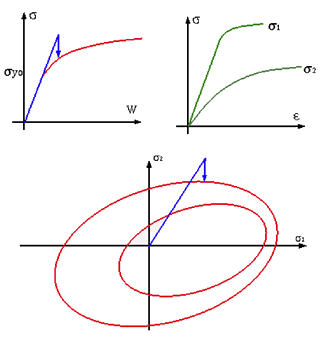
Figure 8. CRASURV Plasticity Hardening
The CRASURV model will allow the simulation of the ductile failure of orthotropic shells. The plastic and failure behaviors are different in tension and in compression. The stress softening may also be introduced in the model to take into account the residual Tsai-Wu stresses. The evolution of CRASURV criteria with hardening and softening works is illustrated in Figure 9.


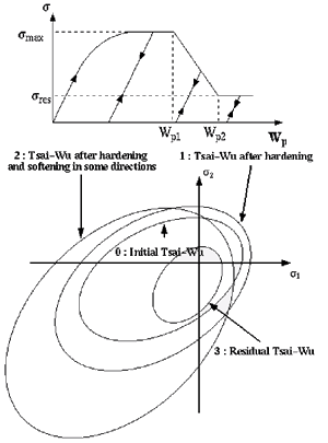
Figure 9. Flow Surface in CRASURV Model

Chang Chang Model

Chang-Chang law 2, 3 incorporated in Radioss is a combination of the standard Tsai-Wu elastic-plastic law and a modified Chang-Chang failure criteria. 4 The affects of damage are taken into account by decreasing stress components using a relaxation technique to avoid numerical instabilities.

Six material parameters are used in the failure criteria:
S 1 MathType@MTEF@5@5@+= feaagKart1ev2aaatCvAUfeBSjuyZL2yd9gzLbvyNv2CaerbuLwBLn hiov2DGi1BTfMBaeXatLxBI9gBaerbd9wDYLwzYbItLDharqqtubsr 4rNCHbGeaGqiVu0Je9sqqrpepC0xbbL8F4rqqrFfpeea0xe9Lq=Jc9 vqaqpepm0xbba9pwe9Q8fs0=yqaqpepae9pg0FirpepeKkFr0xfr=x fr=xb9adbaqaaeGaciGaaiaabeqaamaabaabaaGcbaGaam4uamaaBa aaleaacaaIXaaabeaaaaa@37B5@
Longitudinal tensile strength
S 2 MathType@MTEF@5@5@+= feaagKart1ev2aaatCvAUfeBSjuyZL2yd9gzLbvyNv2CaerbuLwBLn hiov2DGi1BTfMBaeXatLxBI9gBaerbd9wDYLwzYbItLDharqqtubsr 4rNCHbGeaGqiVu0Je9sqqrpepC0xbbL8F4rqqrFfpeea0xe9Lq=Jc9 vqaqpepm0xbba9pwe9Q8fs0=yqaqpepae9pg0FirpepeKkFr0xfr=x fr=xb9adbaqaaeGaciGaaiaabeqaamaabaabaaGcbaGaam4uamaaBa aaleaacaaIXaaabeaaaaa@37B5@
Transverse tensile strength
S 12 MathType@MTEF@5@5@+= feaagKart1ev2aaatCvAUfeBSjuyZL2yd9gzLbvyNv2CaerbuLwBLn hiov2DGi1BTfMBaeXatLxBI9gBaerbd9wDYLwzYbItLDharqqtubsr 4rNCHbGeaGqiVu0Je9sqqrpepC0xbbL8F4rqqrFfpeea0xe9Lq=Jc9 vqaqpepm0xbba9pwe9Q8fs0=yqaqpepae9pg0FirpepeKkFr0xfr=x fr=xb9adbaqaaeGaciGaaiaabeqaamaabaabaaGcbaGaam4uamaaBa aaleaacaaIXaaabeaaaaa@37B5@
Shear strength
C 1 MathType@MTEF@5@5@+= feaagKart1ev2aaatCvAUfeBSjuyZL2yd9gzLbvyNv2CaerbuLwBLn hiov2DGi1BTfMBaeXatLxBI9gBaerbd9wDYLwzYbItLDharqqtubsr 4rNCHbGeaGqiVu0Je9sqqrpepC0xbbL8F4rqqrFfpeea0xe9Lq=Jc9 vqaqpepm0xbba9pwe9Q8fs0=yqaqpepae9pg0FirpepeKkFr0xfr=x fr=xb9adbaqaaeGaciGaaiaabeqaamaabaabaaGcbaGaam4uamaaBa aaleaacaaIXaaabeaaaaa@37B5@
Longitudinal compressive strength
C 2 MathType@MTEF@5@5@+= feaagKart1ev2aaatCvAUfeBSjuyZL2yd9gzLbvyNv2CaerbuLwBLn hiov2DGi1BTfMBaeXatLxBI9gBaerbd9wDYLwzYbItLDharqqtubsr 4rNCHbGeaGqiVu0Je9sqqrpepC0xbbL8F4rqqrFfpeea0xe9Lq=Jc9 vqaqpepm0xbba9pwe9Q8fs0=yqaqpepae9pg0FirpepeKkFr0xfr=x fr=xb9adbaqaaeGaciGaaiaabeqaamaabaabaaGcbaGaam4uamaaBa aaleaacaaIXaaabeaaaaa@37B5@
Transverse compressive strength
β
Shear scaling factor
Where,
1 MathType@MTEF@5@5@+= feaagKart1ev2aaatCvAUfeBSjuyZL2yd9gzLbvyNv2CaerbuLwBLn hiov2DGi1BTfMBaeXatLxBI9gBaerbd9wDYLwzYbItLDharqqtubsr 4rNCHbGeaGqiVu0Je9sqqrpepC0xbbL8F4rqqrFfpeea0xe9Lq=Jc9 vqaqpepm0xbba9pwe9Q8fs0=yqaqpepae9pg0FirpepeKkFr0xfr=x fr=xb9adbaqaaeGaciGaaiaabeqaamaabaabaaGcbaGaaGymaaaa@36B1@
Fiber direction
The failure criterion for fiber breakage is written as:
  • Tensile fiber mode: σ 11 > 0
    (20) e f 2 = ( σ 11 S 1 ) 2 +β ( σ 12 S 12 ) 2 1.0{ 0failed <0elasticplastic MathType@MTEF@5@5@+= feaagKart1ev2aaatCvAUfeBSjuyZL2yd9gzLbvyNv2CaerbwvMCKf MBHbqefqvATv2CG4uz3bIuV1wyUbqedmvETj2BSbqefm0B1jxALjhi ov2DaebbnrfifHhDYfgasaacH8srps0lbbf9q8WrFfeuY=Hhbbf9v8 qqaqFr0xc9pk0xbba9q8WqFfea0=yr0RYxir=Jbba9q8aq0=yq=He9 q8qqQ8frFve9Fve9Ff0dmeaacaGacmGadaWaaiqacaabaiaafaaake aacaWGLbWaa0baaSqaaiaadAgaaeaacaaIYaaaaOGaeyypa0ZaaeWa aeaadaWcaaqaaiabeo8aZnaaBaaaleaacaaIXaGaaGymaaqabaaake aacaWGtbWaaSbaaSqaaiaaigdaaeqaaaaaaOGaayjkaiaawMcaamaa CaaaleqabaGaaGOmaaaakiabgUcaRiabek7aIjaaykW7daqadaqaam aalaaabaGaeq4Wdm3aaSbaaSqaaiaaigdacaaIYaaabeaaaOqaaiaa dofadaWgaaWcbaGaaGymaiaaikdaaeqaaaaaaOGaayjkaiaawMcaam aaCaaaleqabaGaaGOmaaaakiabgkHiTiaaigdacaGGUaGaaGimaiaa ywW7caaMf8+aaiqaaqaabeqaaiabgwMiZkaaicdacaaMe8UaamOzai aadggacaWGPbGaamiBaiaadwgacaWGKbaabaGaeyipaWJaaGimaiaa ykW7caaMe8UaamyzaiaadYgacaWGHbGaam4CaiaadshacaWGPbGaam 4yaiabgkHiTiaadchacaWGSbGaamyyaiaadohacaWG0bGaamyAaiaa dogaaaGaay5Eaaaaaa@74B7@
  • Compressive fiber mode: σ 11 < 0
    (21) e c 2 = ( σ 11 C 1 ) 2 1.0{ 0failed <0elasticplastic MathType@MTEF@5@5@+= feaagKart1ev2aaatCvAUfeBSjuyZL2yd9gzLbvyNv2CaerbwvMCKf MBHbqefqvATv2CG4uz3bIuV1wyUbqedmvETj2BSbqefm0B1jxALjhi ov2DaebbnrfifHhDYfgasaacH8srps0lbbf9q8WrFfeuY=Hhbbf9v8 qqaqFr0xc9pk0xbba9q8WqFfea0=yr0RYxir=Jbba9q8aq0=yq=He9 q8qqQ8frFve9Fve9Ff0dmeaacaGacmGadaWaaiqacaabaiaafaaake aacaWGLbWaa0baaSqaaiaadogaaeaacaaIYaaaaOGaeyypa0ZaaeWa aeaadaWcaaqaaiabeo8aZnaaBaaaleaacaaIXaGaaGymaaqabaaake aacaWGdbWaaSbaaSqaaiaaigdaaeqaaaaaaOGaayjkaiaawMcaamaa CaaaleqabaGaaGOmaaaakiabgkHiTiaaigdacaGGUaGaaGimaiaayw W7caaMf8UaaGjcVlaaywW7caaMf8+aaiqaaqaabeqaaiabgwMiZkaa icdacaaMe8UaamOzaiaadggacaWGPbGaamiBaiaadwgacaWGKbaaba GaeyipaWJaaGimaiaaykW7caaMe8UaamyzaiaadYgacaWGHbGaam4C aiaadshacaWGPbGaam4yaiabgkHiTiaadchacaWGSbGaamyyaiaado hacaWG0bGaamyAaiaadogaaaGaay5Eaaaaaa@6CC2@
For matrix cracking, the failure criterion is:
  • Tensile matrix mode: σ 22 > 0
    (22) e m 2 = ( σ 22 S 2 ) 2 +β( σ 12 S 12 )1.0{ 0failed <0elasticplastic MathType@MTEF@5@5@+= feaagKart1ev2aaatCvAUfeBSjuyZL2yd9gzLbvyNv2CaerbwvMCKf MBHbqefqvATv2CG4uz3bIuV1wyUbqedmvETj2BSbqefm0B1jxALjhi ov2DaebbnrfifHhDYfgasaacH8srps0lbbf9q8WrFfeuY=Hhbbf9v8 qqaqFr0xc9pk0xbba9q8WqFfea0=yr0RYxir=Jbba9q8aq0=yq=He9 q8qqQ8frFve9Fve9Ff0dmeaacaGacmGadaWaaiqacaabaiaafaaake aacaWGLbWaa0baaSqaaiaad2gaaeaacaaIYaaaaOGaeyypa0ZaaeWa aeaadaWcaaqaaiabeo8aZnaaBaaaleaacaaIYaGaaGOmaaqabaaake aacaWGtbWaaSbaaSqaaiaaikdaaeqaaaaaaOGaayjkaiaawMcaamaa CaaaleqabaGaaGOmaaaakiabgUcaRiabek7aInaabmaabaWaaSaaae aacqaHdpWCdaWgaaWcbaGaaGymaiaaikdaaeqaaaGcbaGaam4uamaa BaaaleaacaaIXaGaaGOmaaqabaaaaaGccaGLOaGaayzkaaGaeyOeI0 IaaGymaiaac6cacaaIWaGaaGzbVlaaywW7caaMi8UaaGzbVlaaywW7 daGabaabaeqabaGaeyyzImRaaGimaiaaysW7caWGMbGaamyyaiaadM gacaWGSbGaamyzaiaadsgaaeaacqGH8aapcaaIWaGaaGPaVlaaysW7 caWGLbGaamiBaiaadggacaWGZbGaamiDaiaadMgacaWGJbGaeyOeI0 IaamiCaiaadYgacaWGHbGaam4CaiaadshacaWGPbGaam4yaaaacaGL 7baaaaa@76F0@
  • Compressive matrix mode: σ 22 < 0
    (23) e d 2 = ( σ 22 2 S 12 ) 2 +[ ( C 2 2 S 12 ) 2 1 ] σ 22 C 2 + ( σ 12 S 12 ) 2 1.0{ 0failed <0elasticplastic MathType@MTEF@5@5@+= feaagKart1ev2aaatCvAUfeBSjuyZL2yd9gzLbvyNv2CaerbwvMCKf MBHbqefqvATv2CG4uz3bIuV1wyUbqedmvETj2BSbqefm0B1jxALjhi ov2DaebbnrfifHhDYfgasaacH8srps0lbbf9q8WrFfeuY=Hhbbf9v8 qqaqFr0xc9pk0xbba9q8WqFfea0=yr0RYxir=Jbba9q8aq0=yq=He9 q8qqQ8frFve9Fve9Ff0dmeaacaGacmGadaWaaiqacaabaiaafaaake aacaWGLbWaa0baaSqaaiaadsgaaeaacaaIYaaaaOGaeyypa0ZaaeWa aeaadaWcaaqaaiabeo8aZnaaBaaaleaacaaIYaGaaGOmaaqabaaake aacaaIYaGaam4uamaaBaaaleaacaaIXaGaaGOmaaqabaaaaaGccaGL OaGaayzkaaWaaWbaaSqabeaacaaIYaaaaOGaey4kaSYaamWaaeaada qadaqaamaalaaabaGaam4qamaaBaaaleaacaaIYaaabeaaaOqaaiaa ikdacaWGtbWaaSbaaSqaaiaaigdacaaIYaaabeaaaaaakiaawIcaca GLPaaadaahaaWcbeqaaiaaikdaaaGccqGHsislcaaIXaaacaGLBbGa ayzxaaWaaSaaaeaacqaHdpWCdaWgaaWcbaGaaGOmaiaaikdaaeqaaa GcbaGaam4qamaaBaaaleaacaaIYaaabeaakiabgUcaRaaadaqadaqa amaalaaabaGaeq4Wdm3aaSbaaSqaaiaaigdacaaIYaaabeaaaOqaai aadofadaWgaaWcbaGaaGymaiaaikdaaeqaaaaaaOGaayjkaiaawMca amaaCaaaleqabaGaaGOmaaaakiabgkHiTiaaigdacaGGUaGaaGimai aaywW7caaMf8UaaGzbVpaaceaaeaqabeaacqGHLjYScaaIWaGaaGjb VlaadAgacaWGHbGaamyAaiaadYgacaWGLbGaamizaaqaaiabgYda8i aaicdacaaMc8UaaGjbVlaadwgacaWGSbGaamyyaiaadohacaWG0bGa amyAaiaadogacqGHsislcaWGWbGaamiBaiaadggacaWGZbGaamiDai aadMgacaWGJbaaaiaawUhaaaaa@85CF@
If the damage parameter is equal to or greater than 1.0, the stresses are decreased by using an exponential function to avoid numerical instabilities. A relaxation technique is used by gradually decreasing the stress:(24) [ σ( t ) ]=f( t )[ σ d ( t r ) ] MathType@MTEF@5@5@+= feaagKart1ev2aaatCvAUfeBSjuyZL2yd9gzLbvyNv2CaerbwvMCKf MBHbqefqvATv2CG4uz3bIuV1wyUbqedmvETj2BSbqefm0B1jxALjhi ov2DaebbnrfifHhDYfgasaacH8srps0lbbf9q8WrFfeuY=Hhbbf9v8 qqaqFr0xc9pk0xbba9q8WqFfea0=yr0RYxir=Jbba9q8aq0=yq=He9 q8qqQ8frFve9Fve9Ff0dmeaacaGacmGadaWaaiqacaabaiaafaaake GabaaVqmaadmaabaGaeq4Wdm3aaeWaaeaacaWG0baacaGLOaGaayzk aaaacaGLBbGaayzxaaGaeyypa0JaamOzamaabmaabaGaamiDaaGaay jkaiaawMcaaiabgEHiQmaadmaabaGaeq4Wdm3aaSbaaSqaaiaadsga aeqaaOWaaeWaaeaacaWG0bWaaSbaaSqaaiaadkhaaeqaaaGccaGLOa GaayzkaaaacaGLBbGaayzxaaaaaa@4DC2@

With: f ( t ) = exp ( t t r T ) MathType@MTEF@5@5@+= feaagKart1ev2aaatCvAUfeBSjuyZL2yd9gzLbvyNv2CaerbwvMCKf MBHbqefqvATv2CG4uz3bIuV1wyUbqedmvETj2BSbqefm0B1jxALjhi ov2DaebbnrfifHhDYfgasaacH8srps0lbbf9q8WrFfeuY=Hhbbf9v8 qqaqFr0xc9pk0xbba9q8WqFfea0=yr0RYxir=Jbba9q8aq0=yq=He9 q8qqQ8frFve9Fve9Ff0dmeaacaGacmGadaWaaiqacaabaiaafaaake aacaWGMbWaaeWaaeaacaWG0baacaGLOaGaayzkaaGaeyypa0Jaciyz aiaacIhacaGGWbWaaeWaaeaadaWcaaqaaiaadshacqGHsislcaWG0b WaaSbaaSqaaiaadkhaaeqaaaGcbaGaamivaaaaaiaawIcacaGLPaaa aaa@46A3@ and t t 4 MathType@MTEF@5@5@+= feaagKart1ev2aaatCvAUfeBSjuyZL2yd9gzLbvyNv2CaerbuLwBLn hiov2DGi1BTfMBaeXatLxBI9gBaerbd9wDYLwzYbItLDharqqtubsr 4rNCHbGeaGqiVu0Je9sqqrpepC0xbbL8F4rqqrFfpeea0xe9Lq=Jc9 vqaqpepm0xbba9pwe9Q8fs0=yqaqpepae9pg0FirpepeKkFr0xfr=x fr=xb9adbaqaaeGaciGaaiaabeqaamaabaabaaGcbaGaamiDaiabgw MiZkaadshadaWgaaWcbaGaaGinaaqabaaaaa@3A98@

Where,
t MathType@MTEF@5@5@+= feaagKart1ev2aaatCvAUfeBSjuyZL2yd9gzLbvyNv2CaerbuLwBLn hiov2DGi1BTfMBaeXatLxBI9gBaerbd9wDYLwzYbItLDharqqtubsr 4rNCHbGeaGqiVu0Je9sqqrpepC0xbbL8F4rqqrFfpeea0xe9Lq=Jc9 vqaqpepm0xbba9pwe9Q8fs0=yqaqpepae9pg0FirpepeKkFr0xfr=x fr=xb9adbaqaaeGaciGaaiaabeqaamaabaabaaGcbaGaamiDaaaa@36EF@
Time
t r MathType@MTEF@5@5@+= feaagKart1ev2aaatCvAUfeBSjuyZL2yd9gzLbvyNv2CaerbuLwBLn hiov2DGi1BTfMBaeXatLxBI9gBaerbd9wDYLwzYbItLDharqqtubsr 4rNCHbGeaGqiVu0Je9sqqrpepC0xbbL8F4rqqrFfpeea0xe9Lq=Jc9 vqaqpepm0xbba9pwe9Q8fs0=yqaqpepae9pg0FirpepeKkFr0xfr=x fr=xb9adbaqaaeGaciGaaiaabeqaamaabaabaaGcbaGaamiDamaaBa aaleaacaWGYbaabeaaaaa@3812@
Start time of relaxation when the damage criteria are assumed
τ
Time of dynamic relaxation

[ σ d ( t r ) ] is the stress components at the beginning of damage (for matrix cracking [ σ d ( t r ) ] = ( σ d 22 σ d 12 ) ).

1 Tsai S.W. and Wu E.M., “A general theory of strength for anisotropic materials”, Journal of Composite Materials, 58-80, 1971.
2 Chang, F.K. and Chang, K.Y., “A Progressive Damage Model For Laminated Composites Containing Stress Concentrations”, Journal of Composite Materials, Vol 21, 834-855, 1987.
3 Chang, F.K. and Chang K.Y., “Post-Failure Analysis of Bolted Composites Joints in Tension or Shear-Out Mode Failure”, Journal of Composite Materials, Vol 21, 809-833, 1987.
4 Matzenmiller A. and Schweizerhof K., “Crashworthiness Simulation of composite Structures-a first step with explicit time integration”, Nonlinear Computational Mechanics-State of the Art Ed. p. Wriggers and W. Wagner, 1991.